Descriptives on ideas for Frontier Paper

Abstract

Descriptives on shocks, mental health dynamics and correlation between measures

```{python}
#| label: load-data
import pandas as pd
from plotnine import *
from pathlib import Path


PROJ_ROOT = Path("/Users/st2246/Work/Pilot3")
TIDY = PROJ_ROOT / "data/generated/tidy/main"

in_person = pd.read_stata(TIDY / "07_InPerson_hh_level-hh_id-period.dta", convert_categoricals=False)
in_person = in_person[in_person["period"] == 0] # Drop endline data

mental_health = pd.read_stata(TIDY / "06_Mental_Health-hh_id-period.dta", convert_categoricals=False)

planting = pd.read_stata(f"{TIDY}/29_planting-hh_id-period-crop_id.dta", convert_categoricals=False)
```

Shocks and Mental Health

Types of shock we had and counts

```{python}
#| label: shock-histogram
#| fig-cap: Count of households reporting each shock type at baseline (period 0)

shock_vars = {
    'shock_any':                'Any shock',
    'shock_nonreligious':       'Non-religious\n shock',
    'shock_death_relative':     'Death of\nRelative',
    'shock_death_livestock':    'Death of\nLivestock',
    'shock_natural_disaster':   'Natural\nDisaster',
    'shock_religious_event':    'Religious\nEvent',
    'shock_other':              'Other',
}

color_map = {
    'shock_any': 'purple',
    'shock_religious_event': 'red',
}

shock_counts = (
    pd.DataFrame({
        'shock_type': list(shock_vars.values()),
        'shock_key': list(shock_vars.keys()),
        'count': [in_person[v].eq(1).sum() for v in shock_vars],
    })
    .assign(color=lambda df: df['shock_key'].map(lambda k: color_map.get(k, '#2c7bb6')))
    .sort_values('count', ascending=False)
)

(
    ggplot(shock_counts, aes(x='reorder(shock_type, -count)', y='count', fill='color'))
    + geom_bar(stat='identity', width=0.65)
    + scale_fill_identity()
    + geom_text(aes(label='count'), va='bottom', nudge_y=0.5, size=9)
    + labs(
        x='Shock Type',
        y='Number of Households',
        title='Households Reporting Shocks at Baseline',
    )
    + theme_minimal()
    + theme(
        axis_text_x=element_text(size=9),
        plot_title=element_text(face='bold'),
    )
)
```

Count of households reporting each shock type at baseline (period 0)

Impact on MH at Baseline

```{python}
#| label: shock-mh-regressions
#| output: asis

import statsmodels.formula.api as smf
from stargazer.stargazer import Stargazer
from IPython.display import HTML

# Full-scale MH measures available at baseline (period == 0)
mh_full_vars = ['phq8', 'gad7', 'pss10', 'pswq16', 'diener5', 'cantril_total']

mh_cols = ['hh_id'] + mh_full_vars
mh_bl = mental_health[mental_health['period'] == 0].copy()[mh_cols]

merged = in_person[['hh_id','shock_nonreligious', 'shock_religious_event', 'shock_any']].merge(mh_bl, on='hh_id', how='inner')

models = [
    smf.ols(f'{var} ~ shock_nonreligious', data=merged).fit()
    for var in mh_full_vars
]

models_any = [
    smf.ols(f'{var} ~ shock_any', data=merged).fit()
    for var in mh_full_vars
]

models_religious = [
    smf.ols(f'{var} ~ shock_religious_event', data=merged).fit()
    for var in mh_full_vars
]
```

Non-religious shocks

```{python}
#| label: shock-mh-regressions-nonrelgious
#| output: asis
sg = Stargazer(models)
sg.title('Impact of non-relgious shocks on mental health at baseline')
sg.custom_columns(mh_full_vars, [1] * len(mh_full_vars))
sg.show_model_numbers(False)

sg
```

Impact of non-relgious shocks on mental health at baseline

	phq8	gad7	pss10	pswq16	diener5	cantril_total
Intercept	8.065***	7.244***	19.325***	51.251***	20.729***	11.206***
	(0.150)	(0.138)	(0.152)	(0.236)	(0.225)	(0.129)
shock_nonreligious	-0.323*	-0.207	0.350*	-0.038	-0.251	-0.041
	(0.190)	(0.174)	(0.192)	(0.298)	(0.284)	(0.163)
Observations	2272	2272	2272	2272	2272	2272
R2	0.001	0.001	0.001	0.000	0.000	0.000
Adjusted R2	0.001	0.000	0.001	-0.000	-0.000	-0.000
Residual Std. Error	4.380 (df=2270)	4.017 (df=2270)	4.424 (df=2270)	6.868 (df=2270)	6.543 (df=2270)	3.768 (df=2270)
F Statistic	2.886* (df=1; 2270)	1.406 (df=1; 2270)	3.333* (df=1; 2270)	0.016 (df=1; 2270)	0.780 (df=1; 2270)	0.063 (df=1; 2270)
Note:	*p<0.1; **p<0.05; ***p<0.01

All shocks

```{python}
#| label: shock-mh-regressions-any
#| output: asis

sg = Stargazer(models_any)
sg.title('Impact of any shock on mental health at baseline')
sg.custom_columns(mh_full_vars, [1] * len(mh_full_vars))
sg.show_model_numbers(False)

sg
```

Impact of any shock on mental health at baseline

	phq8	gad7	pss10	pswq16	diener5	cantril_total
Intercept	9.106***	8.000***	19.663***	51.606***	21.482***	12.216***
	(0.259)	(0.238)	(0.264)	(0.409)	(0.389)	(0.223)
shock_any	-1.420***	-1.011***	-0.135	-0.433	-1.039**	-1.183***
	(0.277)	(0.255)	(0.282)	(0.437)	(0.416)	(0.238)
Observations	2272	2272	2272	2272	2272	2272
R2	0.011	0.007	0.000	0.000	0.003	0.011
Adjusted R2	0.011	0.006	-0.000	-0.000	0.002	0.010
Residual Std. Error	4.358 (df=2270)	4.005 (df=2270)	4.427 (df=2270)	6.867 (df=2270)	6.535 (df=2270)	3.748 (df=2270)
F Statistic	26.226*** (df=1; 2270)	15.743*** (df=1; 2270)	0.231 (df=1; 2270)	0.982 (df=1; 2270)	6.244** (df=1; 2270)	24.592*** (df=1; 2270)
Note:	*p<0.1; **p<0.05; ***p<0.01

Religious shocks

```{python}
#| label: shock-mh-regressions-religious
#| output: asis

sg = Stargazer(models_religious)
sg.title('Impact of religious shocks on mental health at baseline')
sg.custom_columns(mh_full_vars, [1] * len(mh_full_vars))
sg.show_model_numbers(False)

sg
```

Impact of religious shocks on mental health at baseline

	phq8	gad7	pss10	pswq16	diener5	cantril_total
Intercept	8.178***	7.269***	19.615***	51.774***	19.858***	12.058***
	(0.173)	(0.159)	(0.175)	(0.271)	(0.258)	(0.147)
shock_religious_event	-0.439**	-0.216	-0.099	-0.762**	0.995***	-1.223***
	(0.204)	(0.187)	(0.206)	(0.320)	(0.304)	(0.174)
Observations	2272	2272	2272	2272	2272	2272
R2	0.002	0.001	0.000	0.003	0.005	0.021
Adjusted R2	0.002	0.000	-0.000	0.002	0.004	0.021
Residual Std. Error	4.378 (df=2270)	4.017 (df=2270)	4.427 (df=2270)	6.860 (df=2270)	6.529 (df=2270)	3.728 (df=2270)
F Statistic	4.629** (df=1; 2270)	1.333 (df=1; 2270)	0.229 (df=1; 2270)	5.691** (df=1; 2270)	10.700*** (df=1; 2270)	49.547*** (df=1; 2270)
Note:	*p<0.1; **p<0.05; ***p<0.01

• Strange, the cantril moves in its own direction
• Religious event good but also other shocks good? (noisy though)
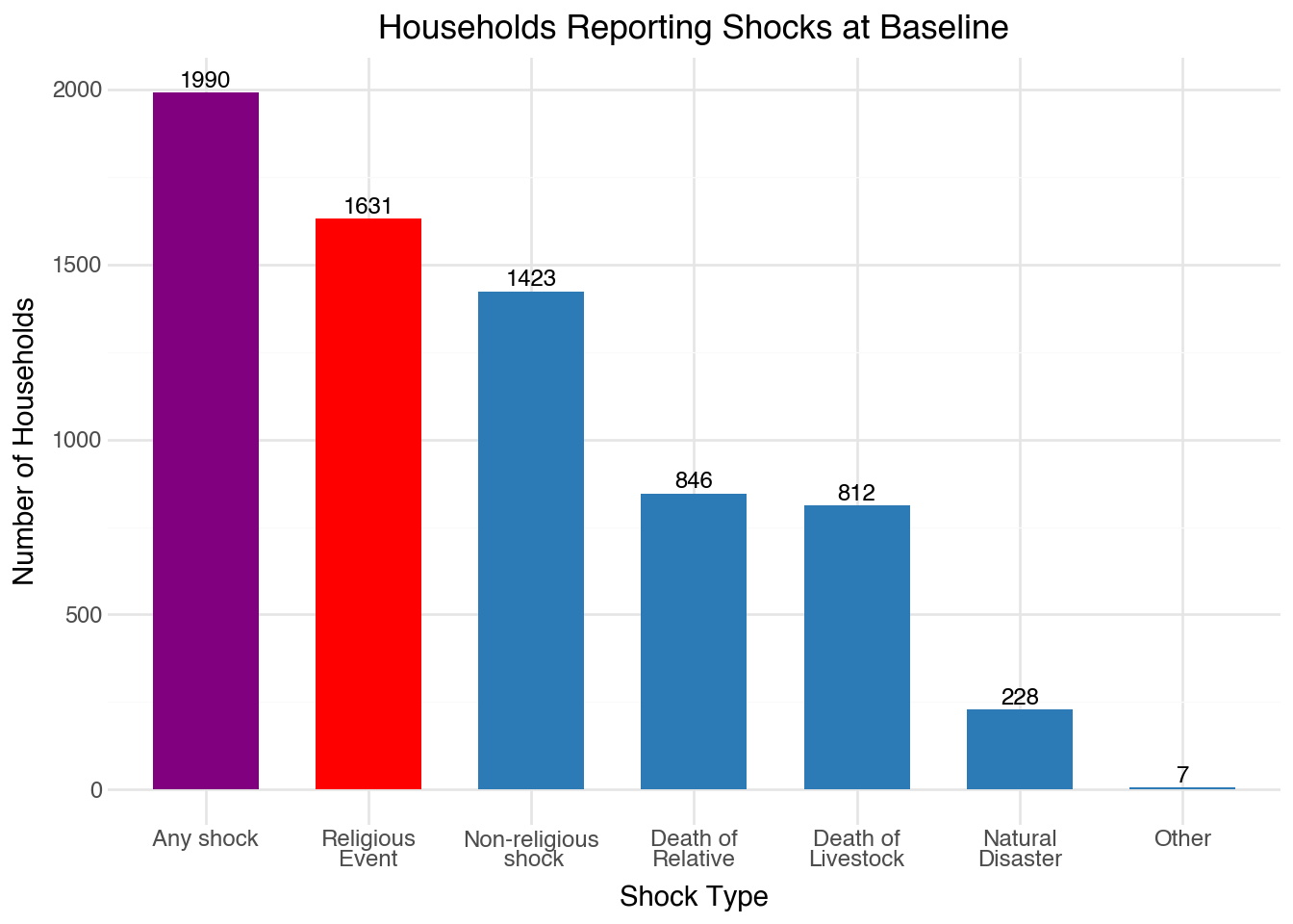
• We do have the sample size to talk about shocks (nearly 50-50 split in who experiences it)

Dynamics and Recovery

```{python}
#| label: shock-period-regressions
#| warning: false
mental_health_vars = ['phq2', 'gad2', 'pss4', 'pswq3']
mh_all = mental_health.copy()[['hh_id', 'period', 'treatment'] + mental_health_vars]
dynamic_data = mh_all.merge(in_person[['hh_id','shock_nonreligious', 'shock_religious_event', 'shock_any']], on='hh_id', how='left')

model_store = {}
for period in range(0, 7):
    model_store[period] = {}
    model_store[period]['nonreligious'] = {}
    for var in mental_health_vars:
         model = smf.ols(f'{var} ~ shock_nonreligious + C(treatment) ', data=dynamic_data[dynamic_data['period'] == period]).fit()
         model_store[period]['nonreligious'][var] = model

    model_store[period]['religious'] = {}
    for var in mental_health_vars:
         model = smf.ols(f'{var} ~ shock_religious_event + C(treatment)  ', data=dynamic_data[dynamic_data['period'] == period]).fit()
         model_store[period]['religious'][var] = model
    model_store[period]['any'] = {}
    for var in mental_health_vars:
        model = smf.ols(f'{var} ~ shock_any + C(treatment) ', data=dynamic_data[dynamic_data['period'] == period]).fit()
        model_store[period]['any'][var] = model
    


# Extract tuple of (coef, se) for shock variable across periods and outcomes
results_store = []
for period in model_store.keys():
    for shock_type in model_store[period].keys():
        for outcome in model_store[period][shock_type].keys():
            model = model_store[period][shock_type][outcome]
            coef = model.params[4]  # Assuming shock variable is the first after intercept
            se = model.bse[4]
            results_store.append({
                'period': period,
                'shock_type': shock_type,
                'outcome': outcome,
                'coef': coef,
                'se': se,
            })
results_clean = pd.DataFrame(results_store) 
results_clean['period'] = results_clean['period'].astype(int)
results_clean['coef'] = results_clean['coef'].astype(float)
results_clean['se'] = results_clean['se'].astype(float)
ojs_define(data=results_clean.to_dict(orient='records')) 
```

```{ojs}
//| panel: sidebar

viewof mental_var = Inputs.select(
  ["phq2", "gad2", "pss4", "pswq3"],
  { label: "Mental scale", value: "phq2" }
)

viewof shock_type = Inputs.select(
  ["nonreligious", "religious", "any"],
  { label: "Shock type", value: "any" }
)
```

filtered = data.filter(d => d.outcome === mental_var && d.shock_type === shock_type)

Plot.plot({
  width: 800,
  height: 500,
  marginLeft: 60,
  grid: true,
  x: { label: "Survey Period" },
  y: { label: "Coefficient Estimate (95% CI)" },
  marks: [
    Plot.ruleY([0]),
    Plot.dot(filtered, { x: "period", y: "coef" }),
    Plot.ruleX(filtered, {
      x: "period",
      y1: d => d.coef - 1.96 * d.se,
      y2: d => d.coef + 1.96 * d.se,
      strokeWidth: 1.5
    })
  ]
})

Mental Health Measures

Correlation heatmap between MH measures broken by period

• Almost no correlation between positives and negatives. It seems like they are almost a separate dimension of mental health.
• Clear link to some mental health measures like depression and anxiety. But correlation with other measures like stress and worry are less strong.

```{python}
#| label: mh-correlation-all
#| warning: false
#| fig-align: center


import numpy as np

# Define list of mental health variables to work with
mental_health_vars = ["phq2", "gad2", "pss4", "pswq3", "diener3", "cantril_total"]

# mental_health_zs = [f"{var}_z_inv" for var in inverted]
mental_health_zs = [f"{var}_z" for var in mental_health_vars]
mental_health_zs += [  # Add composite measures
    "mental_health_index_neg",
]

var_labels = {
    "phq2_z": "PHQ-2\n(Depression)",
    "gad2_z": "GAD-2\n(Anxiety)",
    "pss4_z": "PSS-4\n(Stress)",
    "pswq3_z": "PSWQ-3\n(Worry)",
    "diener3_z": "Diener-3\n(Happiness)",
    "cantril_total_z": "Cantril\n(Life Sat.)",
    "mental_health_index_neg": "Index (Negative MH)",
}


def corr_long(df, vars, label_map=None):
    """Return long-form pairwise correlation DataFrame."""
    corr_mat = df[vars].corr()
    corr_mat.index.name = "var1"
    corr_mat.columns.name = "var2"
    long = corr_mat.stack().reset_index()
    long.columns = ["var1", "var2", "r"]
    long["label"] = long["r"].round(2).astype(str)
    if label_map:
        long["var1"] = long["var1"].map(label_map)
        long["var2"] = long["var2"].map(label_map)
    return long


mh_data = mental_health[["period"] + mental_health_zs].copy()
corr_all = corr_long(mh_data, mental_health_zs, var_labels)

(
    ggplot(corr_all, aes("var1", "var2", fill="r"))
    + geom_tile(color="white", size=0.4)
    + geom_text(aes(label="label"), size=7.5, color="black")
    + scale_fill_gradient2(
        low="#d73027",
        mid="white",
        high="#1a9850",
        midpoint=0,
        limits=[-1, 1],
        name="r",
    )
    + labs(
        title="MH Measure Correlations — All Periods",
        x="",
        y="",
    )
    + theme_minimal()
    + theme(
        axis_text_x=element_text(size=8),
        axis_text_y=element_text(size=8),
        plot_title=element_text(face="bold"),
        figure_size=(10, 5),
    )
)
```

Mental Health Dynamics

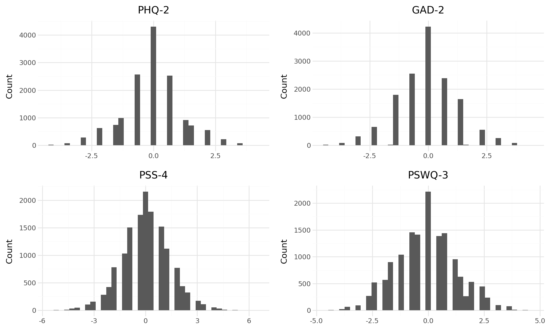
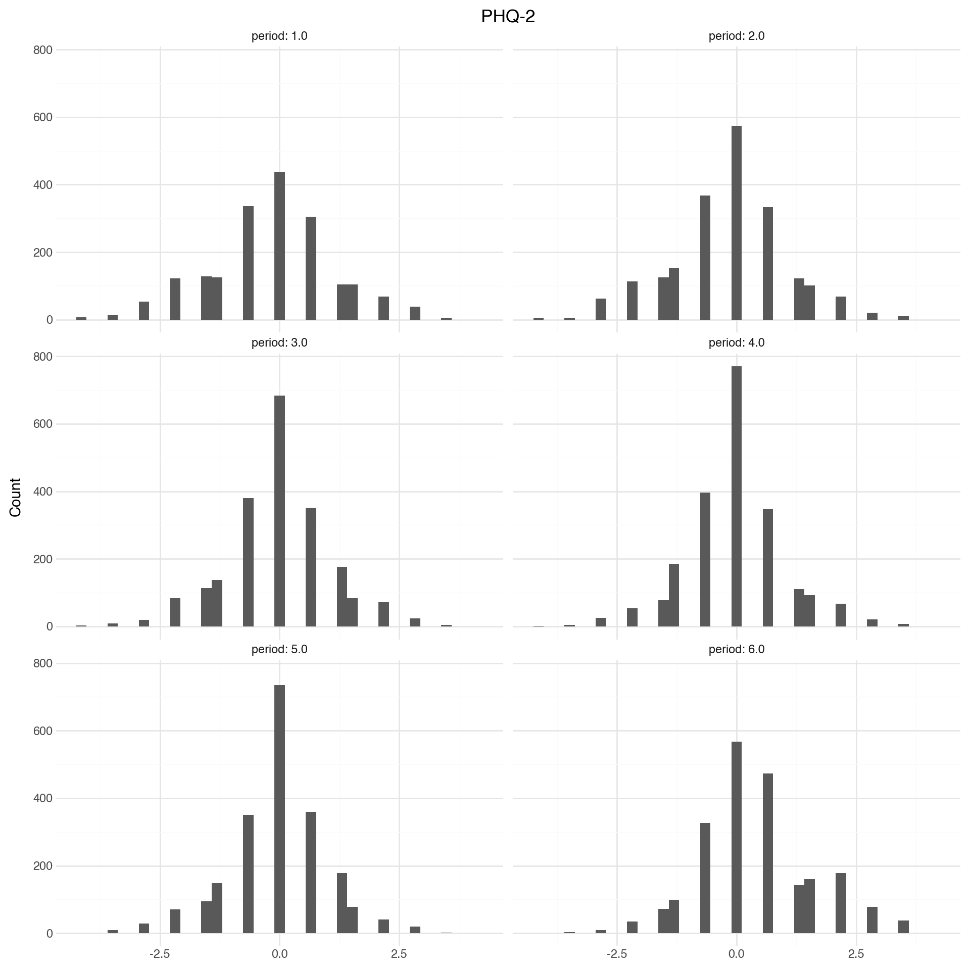
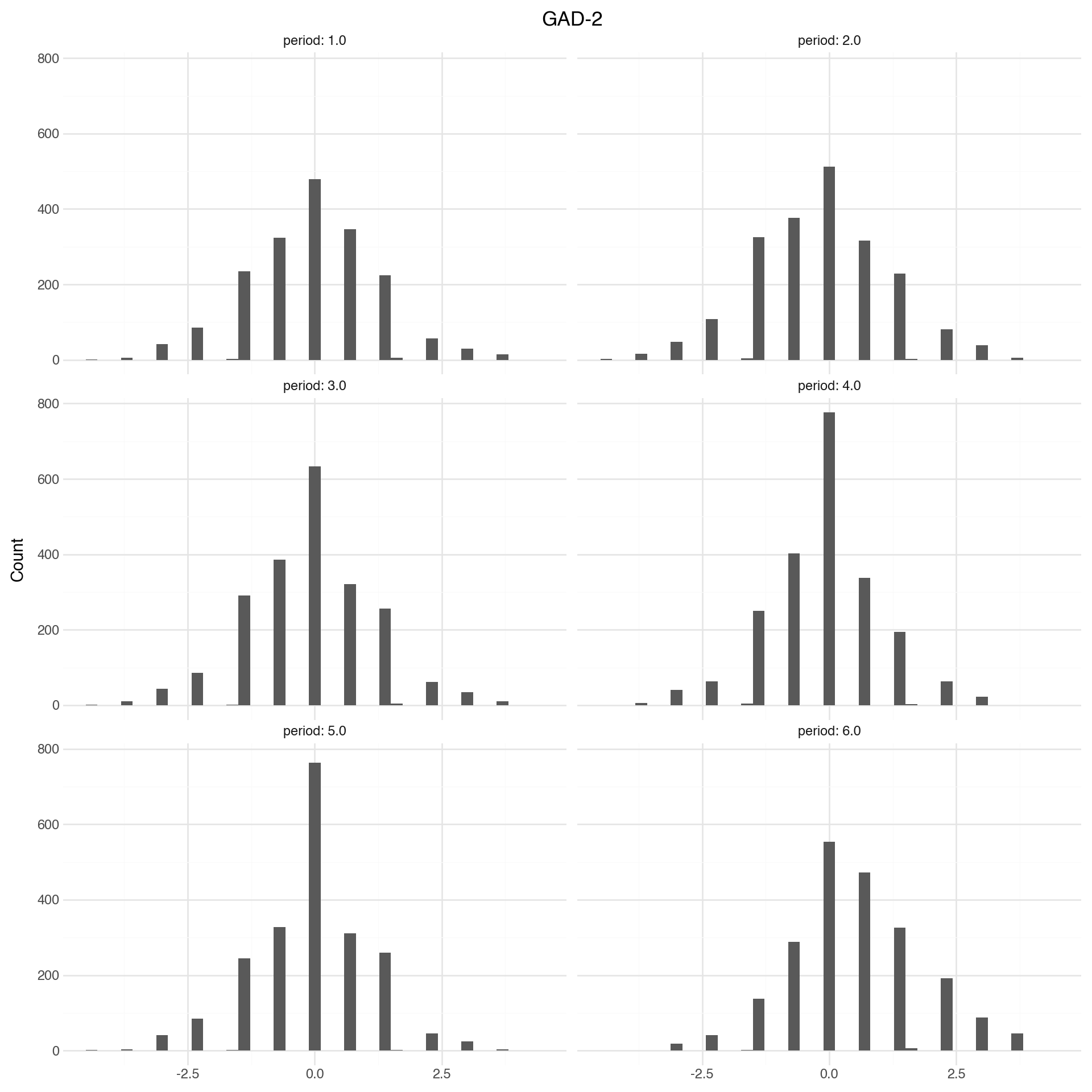
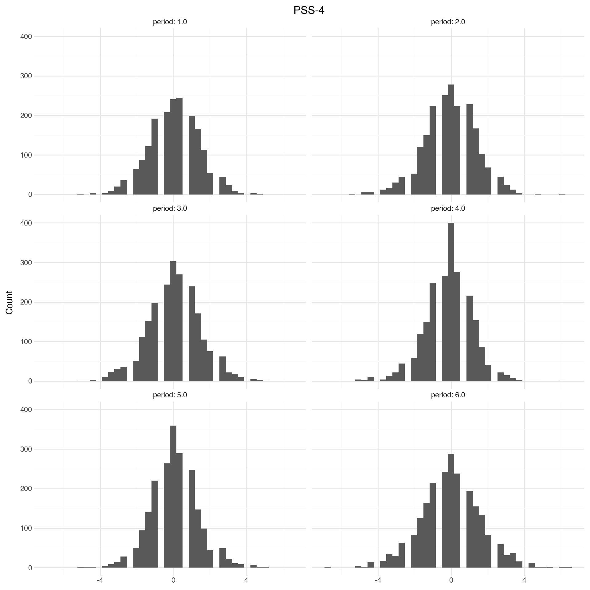
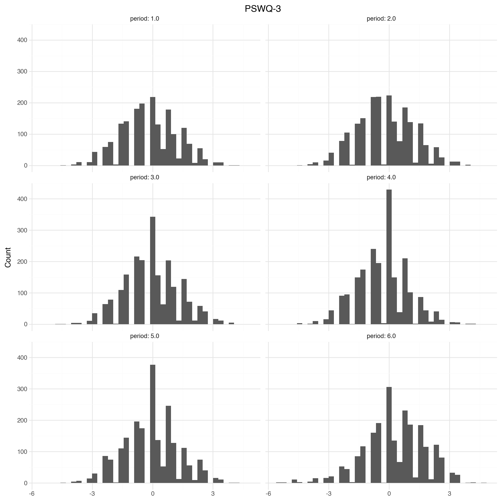
• Measurements are remarkably stable. PHQ and GAD are a lot more stable than the stress and worry measures.
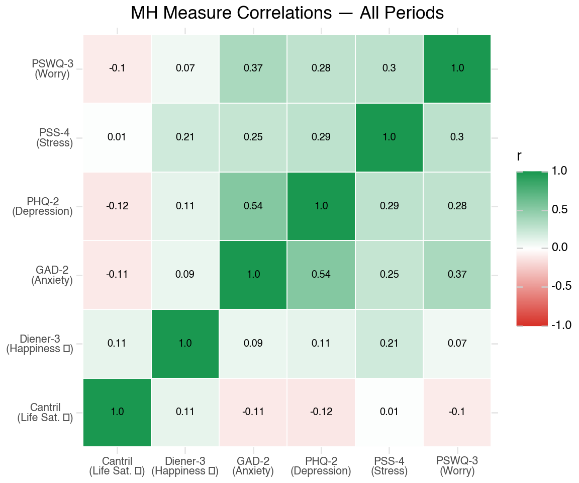
• For the main study, we should consider using the other two measures. This + the correlations not necessarily being super high suggests there is a signal in the different measures

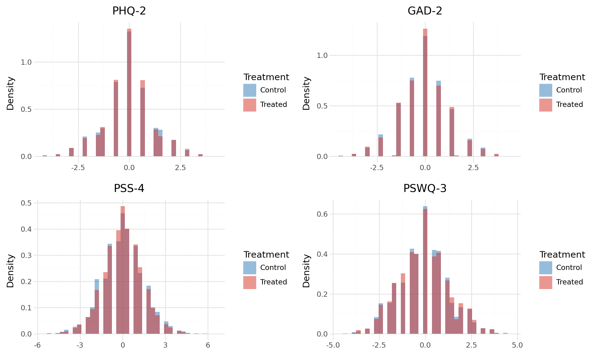
Note

The figures and tables below show how mental health is changing over time. Change is measured as difference in z-scores. Z-scores are computed relative to baseline distribution

```{python}
#| label: mh-dynamics-data
#| fig-align: center


# 2 & 3. Period-over-period change in z-scores, divided by baseline SD → # of SDs changed
dyn = (
    mental_health[
        ["hh_id", "period", "treated"] + [f"{v}_z" for v in mental_health_vars]
    ]
    .sort_values(["hh_id", "period"])
    .copy()
)

for var in mental_health_vars:
    z_col = f"{var}_z"
    diff_col = f"{var}_z_diff"
    dyn[diff_col] = dyn.groupby("hh_id")[z_col].diff()

diff_vars = [f"{v}_z_diff" for v in mental_health_vars]
diff_labels = {
    "phq2_z_diff": "PHQ-2 (Depression)",
    "gad2_z_diff": "GAD-2 (Anxiety)",
    "pss4_z_diff": "PSS-4 (Stress)",
    "pswq3_z_diff": "PSWQ-3 (Worry)",
    "diener3_z_diff": "Diener-3 (Happiness)",
    "cantril_total_z_diff": "Cantril (Life Sat.)",
}

dyn = dyn[dyn["period"] > 0].copy()


def make_changes_distribution(var, title):
    return (
        ggplot(dyn.dropna(subset=[var]), aes(x=var))
        + geom_histogram(bins=40)
        + facet_wrap("~period", ncol=2, labeller="label_both")
        + labs(
            title=f"{title}",
            x="",
            y="Count",
        )
        + theme_minimal()
        + theme(
            figure_size=(10, 10),
        )
    )


def make_changes_distribution_grouped(var, title):
    return (
        ggplot(dyn.dropna(subset=[var]), aes(x=var))
        + geom_histogram(bins=40)
        + labs(
            title=f"{title}",
            x="",
            y="Count",
        )
        + theme_minimal()
        + theme(
            figure_size=(10, 6),
        )
    )


def make_changes_distribution_by_treatment(var, title):
    df = dyn.dropna(subset=[var]).copy()
    df["Treatment"] = df["treated"].map({1: "Treated", 0: "Control"})
    return (
        ggplot(df, aes(x=var, group="Treatment", fill="Treatment"))
        + geom_histogram(
            aes(y=after_stat("density")), bins=40, alpha=0.5, position="identity"
        )
        + scale_fill_manual(values={"Treated": "#d73027", "Control": "#2c7bb6"})
        + labs(
            title=f"{title}",
            x="",
            y="Density",
        )
        + theme_minimal()
        + theme(
            figure_size=(10, 6),
        )
    )
```

```{python}
#| label: mh-dynamics-summary-table

from scipy.stats import median_abs_deviation
from IPython.display import display

rows = []
for var in diff_vars:
    series = dyn[var].dropna()
    row = {
        'Measure': diff_labels[var],
        'Mean': round(series.mean(), 3),
        'SD':   round(series.std(), 3),
        'MAD':  round(median_abs_deviation(series), 3),
    }
    for period, grp in dyn.groupby('period'):
        s = grp[var].dropna()
        row[f'Period {int(period)} SD'] = round(s.std(), 3) if len(s) > 1 else float('nan')
    rows.append(row)

summary_table = pd.DataFrame(rows).set_index('Measure')
summary_table
```

	Mean	SD	MAD	Period 1 SD	Period 2 SD	Period 3 SD	Period 4 SD	Period 5 SD	Period 6 SD	Period 7 SD
Measure
PHQ-2 (Depression)	-0.039	1.205	0.709	1.312	1.230	1.125	1.058	1.075	1.213	1.276
GAD-2 (Anxiety)	-0.054	1.310	0.751	1.301	1.343	1.274	1.120	1.172	1.339	1.368
PSS-4 (Stress)	0.024	1.378	0.852	1.348	1.406	1.411	1.264	1.276	1.536	1.372
PSWQ-3 (Worry)	-0.031	1.362	0.784	1.380	1.386	1.345	1.269	1.351	1.369	1.289
Diener-3 (Happiness)	0.005	1.237	0.884	1.315	1.251	1.243	1.151	1.157	1.264	1.223
Cantril (Life Sat.)	-0.177	0.613	0.000	NaN	NaN	NaN	NaN	NaN	0.613	NaN

```{python}
(
    (
        make_changes_distribution_grouped('phq2_z_diff', 'PHQ-2') 
        | make_changes_distribution_grouped('gad2_z_diff', 'GAD-2')) 
        / (make_changes_distribution_grouped('pss4_z_diff', 'PSS-4') 
        | make_changes_distribution_grouped('pswq3_z_diff', 'PSWQ-3')
    )
)
```

PHQ-2

```{python}
#| label: mh-dynamics-phq2
#| warning: false

make_changes_distribution('phq2_z_diff', 'PHQ-2')
```

GAD-2

```{python}
#| label: mh-dynamics-gad2
#| warning: false
make_changes_distribution('gad2_z_diff', 'GAD-2')
```

PSS-4

```{python}
#| label: mh-dynamics-pss4
#| warning: false
make_changes_distribution('pss4_z_diff', 'PSS-4')
```

PSWQ-3

```{python}
#| label: mh-dynamics-pswq3
#| warning: false
make_changes_distribution('pswq3_z_diff', 'PSWQ-3')
```

By treatment

```{python}
(
    (
        make_changes_distribution_by_treatment('phq2_z_diff', 'PHQ-2')
        | make_changes_distribution_by_treatment('gad2_z_diff', 'GAD-2'))
        / (make_changes_distribution_by_treatment('pss4_z_diff', 'PSS-4')
        | make_changes_distribution_by_treatment('pswq3_z_diff', 'PSWQ-3')
    )
)
```