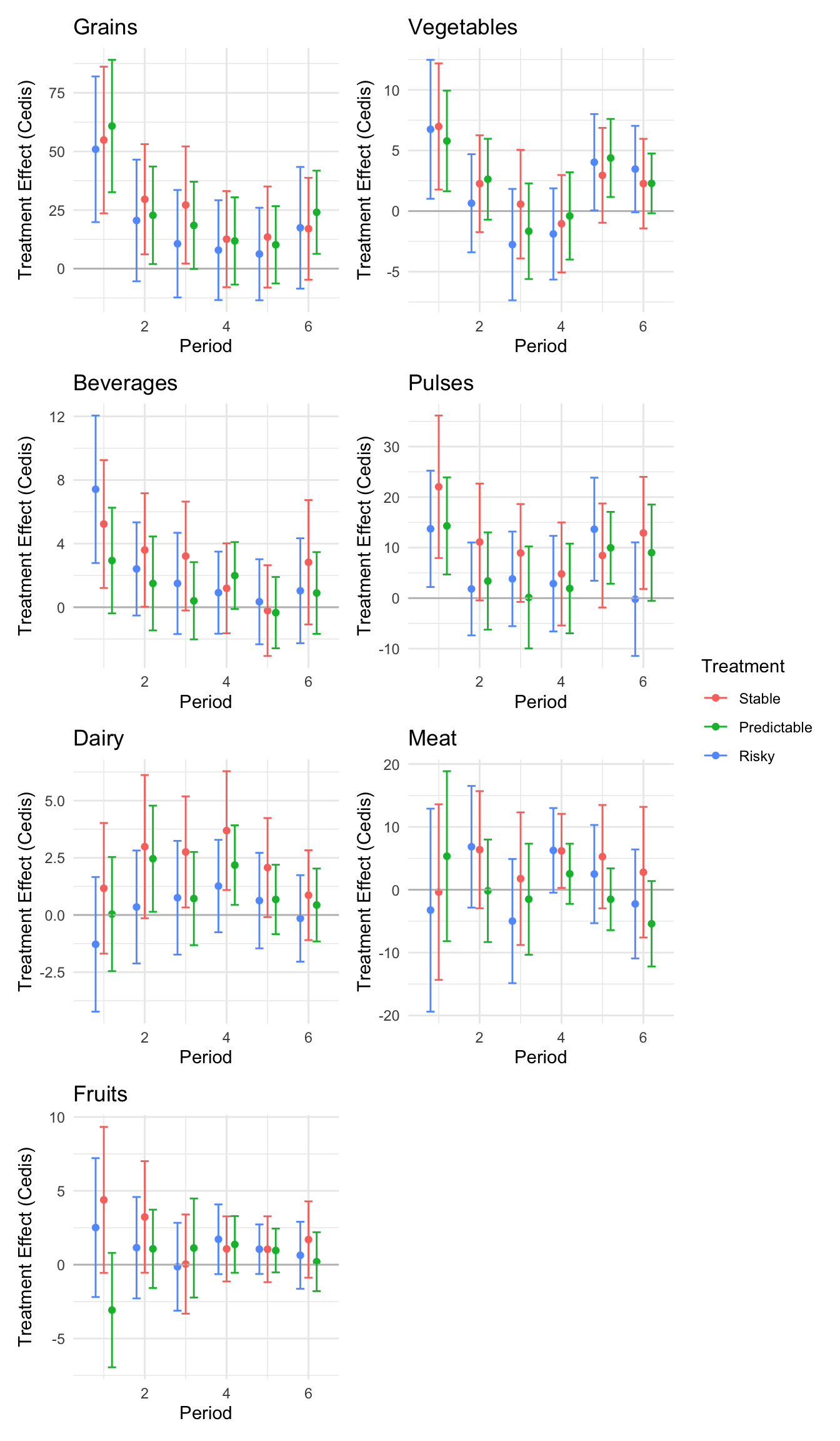
Pre-liminary Results

Published

May 5, 2026

Abstract

First results from the main study survey data

1 Premilinary Results

Code
```{r}
#| message: false
#| warning: false
#| label: load-data

library(tidyverse)
library(fixest)
library(haven)
library(kableExtra)
library(modelsummary)
library(ggplot2)
library(patchwork)
library(DescTools)
library(broom)
library(tibble)
library(dplyr)
library(tidyr)
library(haven)

setFixest_nthreads(1)

conflicted::conflict_prefer("select", "dplyr")
conflicted::conflict_prefer("filter", "dplyr")

theme_set(theme_minimal())


# To refresh data, first run the do file at:
###### "/Users/st2246/Work/Pilot3/code/tidy_run_main.do"
# Then run python file:
##### /Users/st2246/Work/Pilot3/code/pipeline/load.py
df <- read_dta("/Users/st2246/Work/Pilot3/data/generated/main/transform/30_merged_panel-hh_id-period.dta") %>%
    mutate(
        treatment = as.factor(treatment),
        treatment_split = as.factor(treatment_split),
        treatment_balanced = as.factor(treatment_balanced),
        enum_id = as.factor(enum_id),
        # Make sure draw is non-empty for control arms too
        draw_realized = ifelse(treatment == 0, "C", draw_realized),
        draw_imputed = ifelse(treatment == 0, "C", draw_imputed),
        draw_imputed_lag1 = ifelse(treatment == 0, "C", draw_imputed_lag1),
        draw_realized_lag1 = ifelse(treatment == 0, "C", draw_realized_lag1),
        pass_bags = if_else(is.na(pass_bags), 0, pass_bags),
        study_income = as.numeric(pass_bags * 12),
        study_income = if_else(treatment == 0, 0, study_income),
        study_income = if_else(pickup_completed == 0, 0, study_income),
        # high = draw == "H"
        hh_size = as.numeric(hh_size),
        hh_id = as.factor(hh_id)
    ) %>%
    group_by(hh_id) %>%
    mutate(
        early_high_count = sum(period %in% c(1, 2, 3) & draw_imputed == "H", na.rm = TRUE)
    ) %>%
    ungroup() %>%
    mutate(
        treatment_timing = case_when(
            as.integer(as.character(treatment)) == 0 ~ 0,
            as.integer(as.character(treatment)) == 1 ~ 1,
            as.integer(as.character(treatment)) == 2 & early_high_count >= 2 ~ 2,
            as.integer(as.character(treatment)) == 2 & early_high_count <= 1 ~ 3,
            as.integer(as.character(treatment)) == 3 & early_high_count >= 2 ~ 4,
            as.integer(as.character(treatment)) == 3 & early_high_count <= 1 ~ 5
        ),
        treatment_timing = factor(treatment_timing, levels = 0:5)
    )

# Food consumption categories
food_categories <- c("grains", "veges", "bevs", "pulses", "dairy", "meat", "fruits")
# Note: we only have fruit consumption, not purchases since we don't ask for itemized fruit purchases in the phone survey
consumption_category_vars <- paste0("food_consumption_", food_categories, "_99") 
#purchase_category_vars <- paste0("food_purchase_", food_categories, "_99")

# Define variables to analyze
variables <- c(
    "loan_total_outstanding_99",
    "loans_taken",
    "loan_total_payment",
    "food_consumption_total_99",
    "food_consumption_total_phone_99",
    "food_purchase_total_phone_99",
    "food_purchase_total_99",
    "total_consumption_99",
    "expenditure_total_nonfood_99",
    "days_worked_corrected",
    "money_work_corrected_99",
    "days_worked_p_corrected",
    "money_earn_p_corrected",
    "work_engaged_p_corrected",
    "working_adults_corrected",
    "gad2_z",
    "phq2_z",
    "dd_hdds_z",
    "fi_index_anderson",
    "svg_current_savings_99",
    "svg_savings_flow_99",
    "total_income_99",
    "asset_sales_99",
    "asset_purchases_99",
    "asset_net_99",
    "money_work_99",
    "days_worked",
    "working_adults",
    consumption_category_vars
)


# Make basic tables using modelsummary and kableExtra to show results
variableLabels <- c(
    "loan_total_outstanding_99" = "Loans taken",
    "loans_taken" = "Number of Loans Taken",
    "loan_total_payment" = "Loan repayments",
    "food_consumption_total_99" = "Food Consumption Total",
    "food_consumption_total_phone_99" = "Food Consumption (Phone Items)",
    "food_purchase_total_phone_99" = "Food Purchase (Phone Items)",
    "food_purchase_total_99" = "Food Purchase Total",
    "total_consumption_99" = "Total Consumption",
    "expenditure_total_nonfood_99" = "Non-Food Expenditure",
    "days_worked_corrected" = "Days Worked",
    "money_work_corrected_99" = "Income from Work",
    "days_worked_p_corrected" = "Days Worked (Participant)",
    "money_earn_p_corrected" = "Money Total (Participant)",
    "work_engaged_p_corrected" = "Working? (Participant)",
    "working_adults_corrected" = "Working Adults",
    "gad2_z" = "GAD-2 Z-Score",
    "phq2_z" = "PHQ-2 Z-Score",
    "dd_hdds_z" = "HDDS Z-Score",
    "fi_index_anderson" = "FI Index",
    "svg_current_savings_99" = "Current Savings",
    "svg_savings_flow_99" = "Savings Flow",
    "total_income_99" = "Total Income",
    "asset_sales_99" = "Asset Sales",
    "asset_purchases_99" = "Asset Purchases",
    "asset_net_99" = "Asset Net",
    "money_work_99" = "Income from Work",
    "days_worked" = "Days Worked",
    "working_adults" = "Working Adults",
    "food_consumption_grains_99" = "Grains",
    "food_consumption_veges_99" = "Vegetables",
    "food_consumption_bevs_99" = "Beverages",
    "food_consumption_pulses_99" = "Pulses",
    "food_consumption_dairy_99" = "Dairy",
    "food_consumption_meat_99" = "Meat",
    "food_consumption_fruits_99" = "Fruits",
    "food_purchase_grains_99" = "Grains",
    "food_purchase_veges_99" = "Vegetables",
    "food_purchase_bevs_99" = "Beverages",
    "food_purchase_pulses_99" = "Pulses",
    "food_purchase_dairy_99" = "Dairy",
    "food_purchase_meat_99" = "Meat",
    "food_purchase_fruits_99" = "Fruits"
)
# Make baseline labels by iterating through variableLabels and adding _bl to the variable name and "Baseline" to the variable label
variableLabelsBl <- setNames(paste("Baseline", variableLabels), paste0(names(variableLabels), "_bl"))


# Calculate control group baseline means and SDs
control_baseline_stats <- df %>%
    filter(treatment == 0, period == 0) %>%
    summarise(across(
        all_of(setdiff(variables, c("phq2_z", "gad2_z"))),
        list(
            mean = ~ mean(.x, na.rm = TRUE),
            sd = ~ sd(.x, na.rm = TRUE)
        ),
        .names = "{.col}_{.fn}"
    ))


# Create standardized versions of variables using control baseline stats
df <- df %>%
    mutate(across(
        all_of(setdiff(variables, c("phq2_z", "gad2_z"))),
        ~ (.x - control_baseline_stats[[paste0(cur_column(), "_mean")]]) /
            control_baseline_stats[[paste0(cur_column(), "_sd")]],
        .names = "{.col}_z"
    ))


variables_and_z <- c(variables, paste0(setdiff(variables, c("phq2_z", "gad2_z")), "_z"))

# Create baseline values using filter + join approach
baseline_df <- df %>%
    filter(period == 0) %>%
    select(hh_id, all_of(c(variables, variables_and_z))) %>%
    rename_with(~ paste0(.x, "_bl"), .cols = -hh_id)

df <- df %>%
    left_join(baseline_df, by = "hh_id")
```
Code
```{r}
#| message: false
#| warning: false
#| label: run-regressions

# Function to run regressions for a variable
run_regressions <- function(
    var,
    varLabel = variableLabels[var],
    reg_data = df,
    fe_spec = "| district_id + period + wave + enum_id + day_of_week + cohort",
    fe_spec_endline = "| district_id + wave + enum_id + day_of_week + cohort",
    controls = paste0(var, "_bl + hh_size + census_wealth_index")) {

    reg_data_bl <- reg_data 
    reg_data <- reg_data %>%
        filter(period > 0)


    # By Treatment groups
    group_reg <- feols(as.formula(paste0(var, " ~ ", controls, " + i(treatment) ", fe_spec)),
        cluster = "hh_id",
        data = reg_data
    )

    group_reg_timing <- feols(as.formula(paste0(var, " ~ ", controls, " + i(treatment_timing) ", fe_spec)),
        cluster = "hh_id",
        data = reg_data %>% filter(period < 6)
    )

    # By Treatment groups - including baseline
    group_reg_with_baseline <- feols(as.formula(paste0(var, " ~ ", controls, " + i(treatment) ", fe_spec)),
        cluster = "hh_id",
        data = reg_data_bl
    )

    group_reg_no_endline <- feols(as.formula(paste0(var, " ~ ", controls, " + i(treatment) ", fe_spec)),
        cluster = "hh_id",
        data = reg_data %>% filter(period < 6)
    ) 

    # By Treatment groups - balanced_risky
    group_reg_balanced <- feols(as.formula(paste0(var, " ~ ", controls, " + i(treatment_balanced) ", fe_spec)),
        cluster = "hh_id",
        data = reg_data
    )
    # By Treatment groups - balanced_risky
    group_reg_split <- feols(as.formula(paste0(var, " ~ ", controls, " + i(treatment_split) ", fe_spec)),
        cluster = "hh_id",
        data = reg_data
    )

    income_reg <- feols(as.formula(paste0(var, " ~ ", controls, " + study_income ", fe_spec)),
        cluster = "hh_id",
        data = reg_data
    )

    income_and_treatment_reg <- feols(as.formula(paste0(var, " ~ ", controls, " + i(treatment) + study_income ", fe_spec)),
        cluster = "hh_id",
        data = reg_data
    )

    income_treatment_interaction_reg <- feols(as.formula(paste0(var, " ~ ", controls, " + i(treatment) * study_income ", fe_spec)),
        cluster = "hh_id",
        data = reg_data,
        collin.tol = 1e-5
    )

    draw_imputed_reg <- feols(as.formula(paste0(var, " ~ ", controls, " + i(draw_imputed, ref = 'C') + unpredictable ", fe_spec)),
        cluster = "hh_id",
        data = reg_data
    )

    draw_imputed_with_lag_reg <- feols(as.formula(paste0(var, " ~ ", controls, " + i(draw_imputed, ref = 'C') + i(draw_imputed_lag1, ref = 'C') + unpredictable ", fe_spec)),
        cluster = "hh_id",
        data = reg_data
    )

    draw_realized_reg <- feols(as.formula(paste0(var, " ~ ", controls, " + i(draw_realized, ref = 'C') + unpredictable ", fe_spec)),
        cluster = "hh_id",
        data = reg_data %>% filter(draw_realized != "")
    )

    draw_realized_with_lag_reg <- feols(as.formula(paste0(var, " ~ ", controls, " + i(draw_realized, ref = 'C') + i(draw_realized_lag1, ref = 'C') + unpredictable ", fe_spec)),
        cluster = "hh_id",
        data = reg_data %>% filter(draw_realized != "" & draw_realized_lag1 != "")
    )

    # By Treatment groups -> Using balanced panel of people who completed all surveys
    balanced_panel_reg <- feols(as.formula(paste0(var, " ~ ", controls, " + i(treatment) ", fe_spec)),
        cluster = "hh_id",
        data = reg_data %>% filter(completed_all_surveys == 1)
    )

    endline_only <- feols(as.formula(paste0(var, " ~ ", controls, " + i(treatment) ", fe_spec_endline)),
        cluster = "community_id",
        data = reg_data %>% filter(period == 6)
    )

    treated_v_control <- feols(as.formula(paste0(var, " ~ ", controls, " + treated ", fe_spec)),
        cluster = "hh_id",
        data = reg_data
    )

    treated_v_control_endline <- feols(as.formula(paste0(var, " ~ ", controls, " + treated ", fe_spec_endline, " + enum_id")),
        cluster = "community_id",
        data = reg_data %>% filter(period == 6)
    )

    # Create named list using simple numeric names to avoid HTML encoding
    return(setNames(
        list(
            group_reg, group_reg_timing, group_reg_balanced, group_reg_split,
            income_reg, income_and_treatment_reg, income_treatment_interaction_reg,
            draw_imputed_reg, draw_imputed_with_lag_reg, draw_realized_reg,
            draw_realized_with_lag_reg, balanced_panel_reg, endline_only,
            treated_v_control, treated_v_control_endline, group_reg_with_baseline, group_reg_no_endline
        ),
        c(
            varLabel,
            paste0(varLabel, " - Anticipation Effect"),
            paste0(varLabel, " - Balanced Risky"),
            paste0(varLabel, " - Split Risky"),
            paste0(varLabel, " - Income"),
            paste0(varLabel, " - Income + Arm"),
            paste0(varLabel, " - Income X Arm"),
            paste0(varLabel, " - Imputed Draw"),
            paste0(varLabel, " - Imputed Draw with Lag"),
            paste0(varLabel, " - Realized Draw"),
            paste0(varLabel, " - Realized Draw with Lag"),
            paste0(varLabel, " - Balanced Panel"),
            paste0(varLabel, " - Endline Only"),
            paste0(varLabel, " - Treated vs Control"),
            paste0(varLabel, " - Treated vs Control (Endline Only)"),
            paste0(varLabel, " - Baseline Included"),
            paste0(varLabel, " - Excluding Endline")
        )
    ))
}

# Run regressions on all dv's specified in variables
models <- map(variables, run_regressions) %>%
    set_names(variables)


# Make a list of _z variables (std version of dv's)
zVariables <- c(paste0(setdiff(variables, c("phq2_z", "gad2_z")), "_z"), "gad2_z", "phq2_z")
# Run regressions on them
# The results are used for effect plots below
z_models <- map(zVariables, run_regressions) %>%
    set_names(zVariables)
```
Code
```{r}
allLabels <- c(
    variableLabels,
    # variableLabelsBl,
    "treatment" = "Arm",
    "treated" = "Treated",
    # "period::1" = "Period 1",
    # "period::2" = "Period 2",
    # "period::3" = "Period 3",
    # "period::4" = "Period 4",
    # "period::5" = "Period 5",
    # "period::6" = "Endline",
    "treatment::1" = "Stable",
    "treatment::2" = "Predictable",
    "treatment::3" = "Risky",
    "treatment_balanced::1" = "Stable",
    "treatment_balanced::2" = "Predictable",
    "treatment_balanced::3" = "Risky (Balanced)",
    "treatment_split::1" = "Stable",
    "treatment_split::2" = "Predictable",
    "treatment_split::3" = "Risky Medium",
    "treatment_split::4" = "Risky High",
    "treatment_split::5" = "Risky Low",
    "treatment_timing::1" = "Stable",
    "treatment_timing::2" = "Predictable Early",
    "treatment_timing::3" = "Predictable Late",
    "treatment_timing::4" = "Risky Early",
    "treatment_timing::5" = "Risky Late",
    "draw_realized::H" = "High Draw",
    "draw_realized::M" = "Medium Draw",
    "draw_realized::L" = "Low Draw",
    "draw_realized_lag1::H" = "High Draw previous period",
    "draw_realized_lag1::M" = "Medium Draw previous period",
    "draw_realized_lag1::L" = "Low Draw previous period",
    "draw_imputed::H" = "High Draw",
    "draw_imputed::M" = "Medium Draw",
    "draw_imputed::L" = "Low Draw",
    "draw_imputed_lag1::H" = "High Draw previous period",
    "draw_imputed_lag1::M" = "Medium Draw previous period",
    "draw_imputed_lag1::L" = "Low Draw previous period",
    "study_income" = "Study Income",
    "study_income:treatment::1" = "Stable × Study Income",
    "study_income:treatment::2" = "Predictable × Study Income",
    "study_income:treatment::3" = "Risky × Study Income"
    # add labels for interaction between study income and arm
)

makeTable <- function(models) {
    table <- modelsummary(models,
        escape = FALSE,
        coef_map = allLabels,
        output = "kableExtra",
        estimate = "{estimate}{stars}",
        statistic = "{std.error} ({conf.low}, {conf.high})",
        coef_omit = NULL,
        coef_omit_sources = FALSE,
        stars = c(`***` = 0.01, `**` = 0.05, `*` = 0.1),
        gof_map = tribble(
            ~raw, ~clean, ~fmt,
            "nobs", "Observations", 0,
            "FE", "Community FE", 1,
        )
    ) %>%
        kable_classic(full_width = F, html_font = "Cambria", fixed_thead = T)
    table
}
```
Code
```{r}
#| message: false
#| warning: false
#| label: regression-plot-functions

# Function to run regressions for a variable
generate_coeff_df <- function(estimate_data, var) {
    # Get the label for the variable
    varLabel <- variableLabels[var]
    # Define common controls specification
    controls <- paste0(var, "_bl + hh_size")

    period <- c(0, 1, 2, 3, 4, 5, 6)
    estimate_df <- map(period, ~
        tidy(
            feols(as.formula(paste0(var, " ~ ", controls, " + i(treatment) | community_id")),
                cluster = "community_id",
                data = estimate_data %>% filter(period == .x)
            ),
            conf.int = TRUE
        ))
    # Aggreagte estimate_df into one, adding a period column
    estimate_df <- bind_rows(estimate_df, .id = "period") %>%
        filter(str_detect(term, "treatment")) %>%
        filter(period != 1) %>%
        mutate(
            period = as.numeric(period) - 1,
            treatment = case_when(
                term == "treatment::1" ~ "Stable",
                term == "treatment::2" ~ "Predictable",
                term == "treatment::3" ~ "Risky",
            ),
            # add jitter to period for plotting based on treatment
            period = case_when(
                treatment == "Stable" ~ period - 0.2,
                treatment == "Predictable" ~ period,
                treatment == "Risky" ~ period + 0.2,
            )
        ) %>%
        select(!c(term))

    estimate_df
}

effects_grapher <- function(data, ylabel) {
    ggplot(data, aes(x = period, y = estimate, group = treatment, color = treatment)) +
        geom_point() +
        geom_hline(yintercept = 0, color = "grey") +
        geom_errorbar(aes(ymin = conf.low, ymax = conf.high)) +
        ylab(ylabel) +
        xlab("Period")
}
```
Note

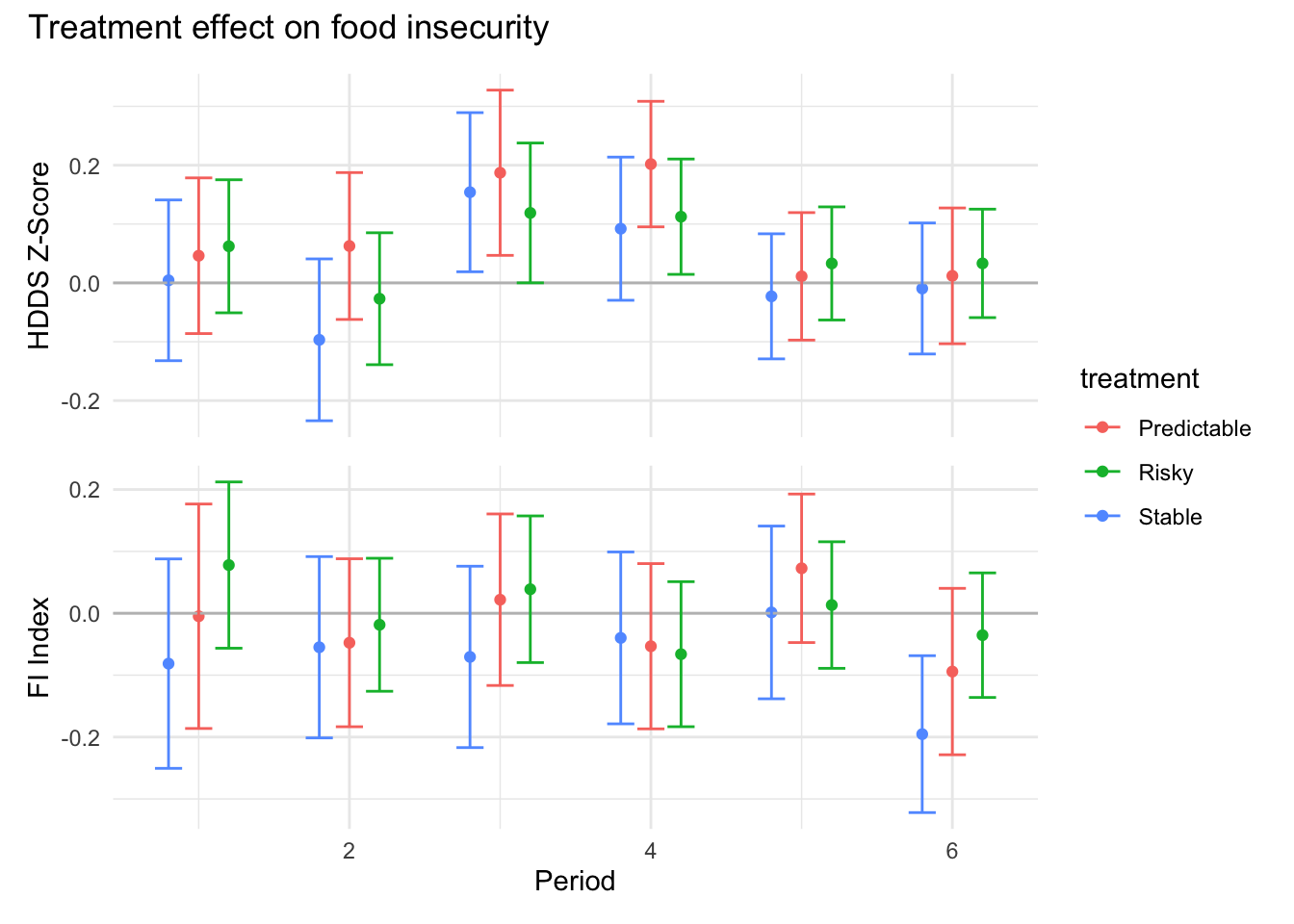
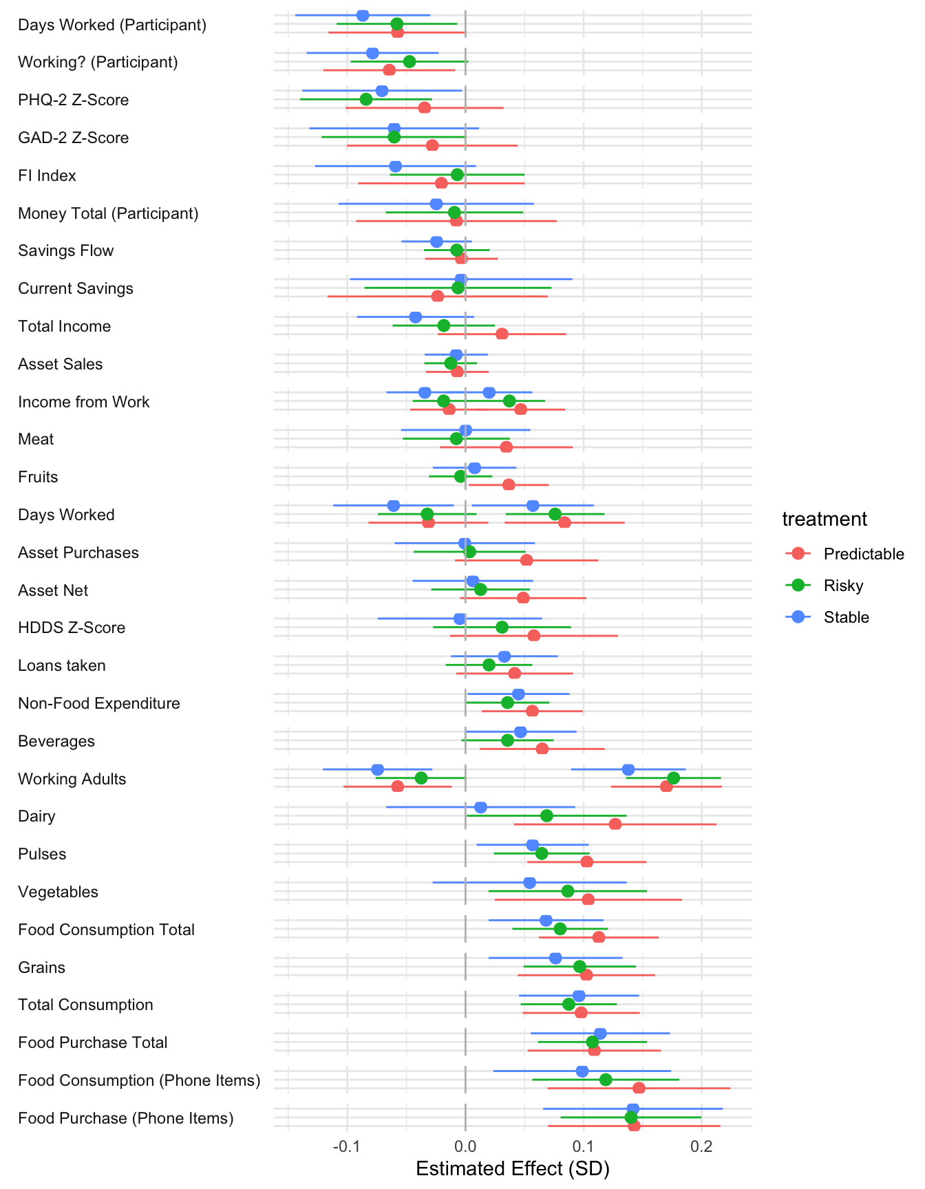
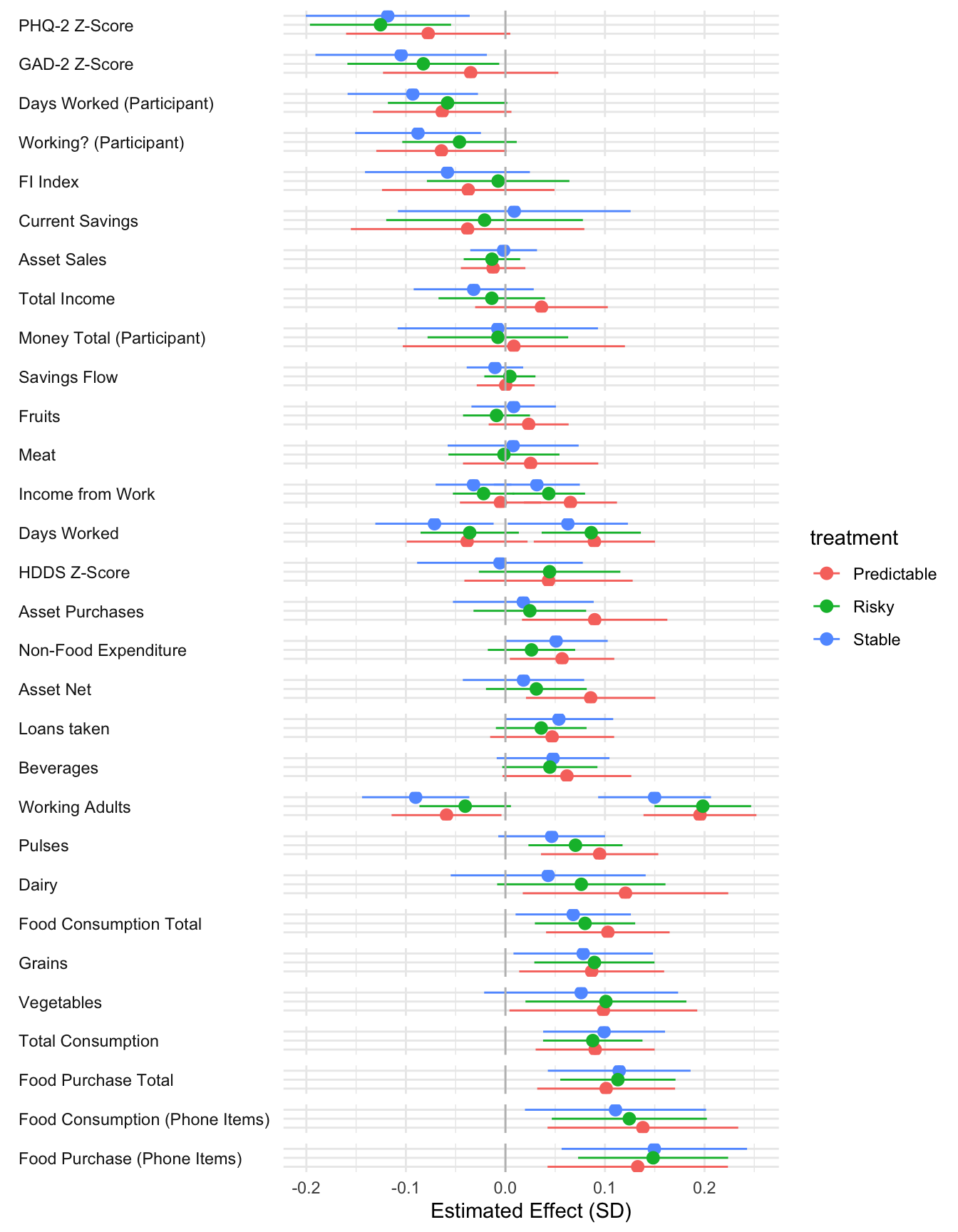
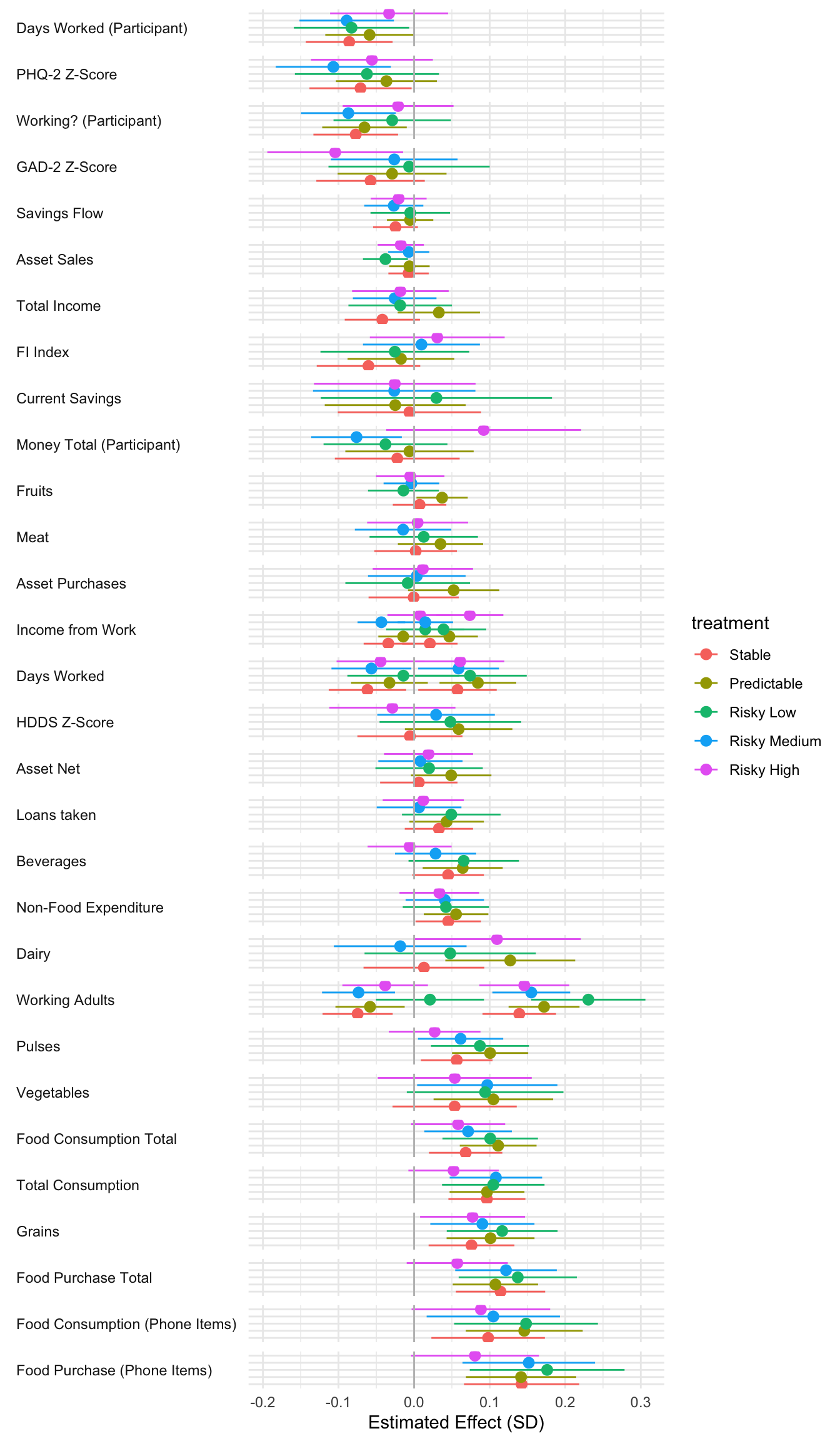
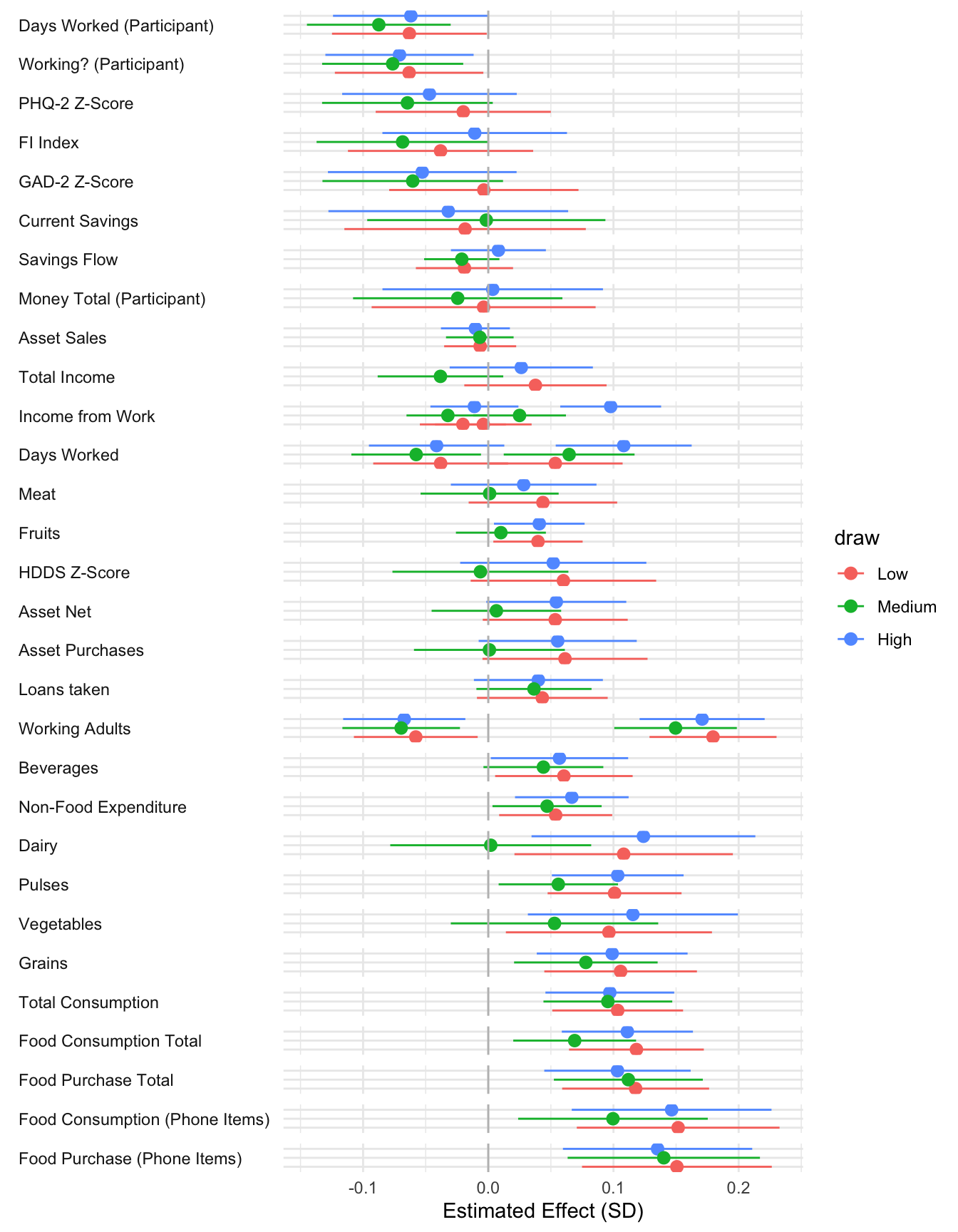
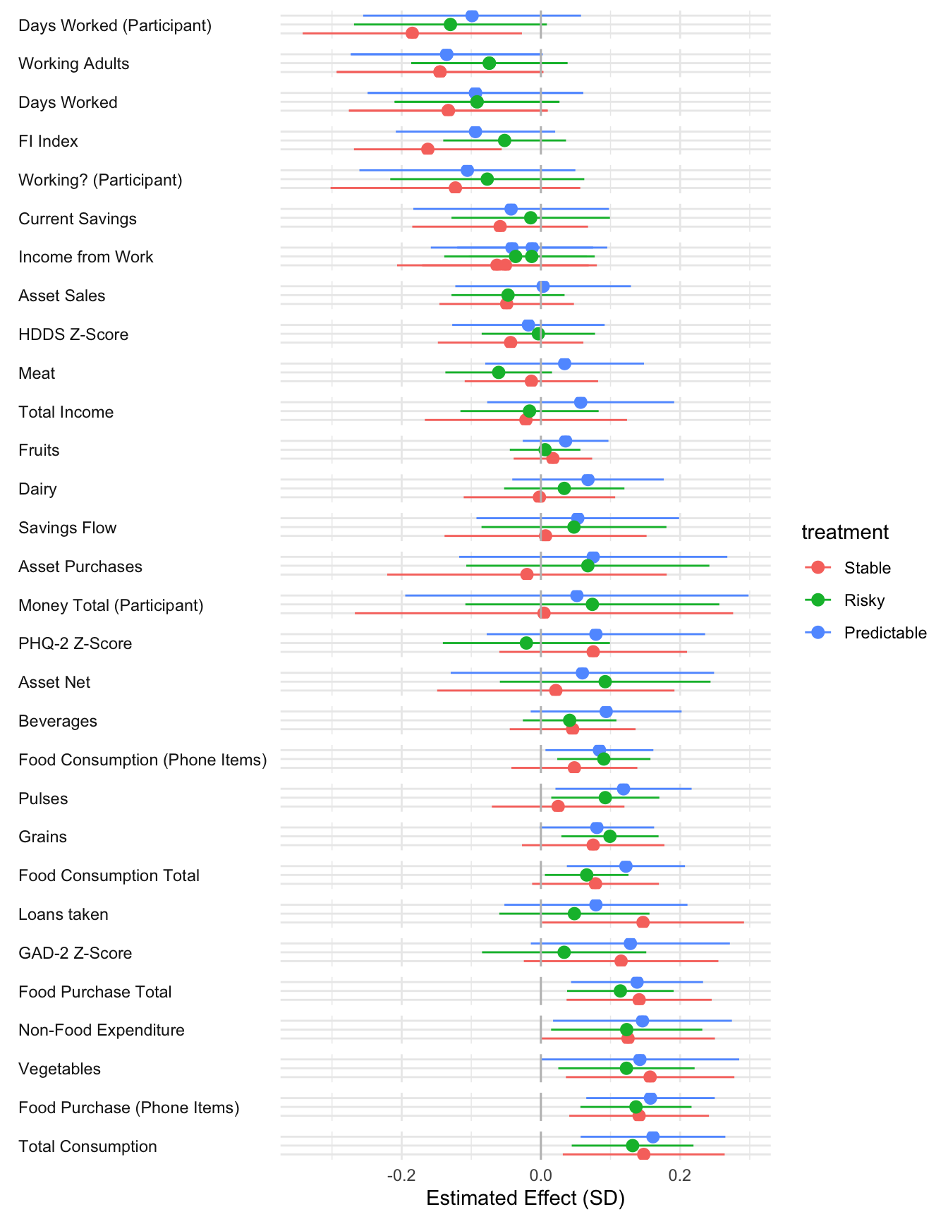
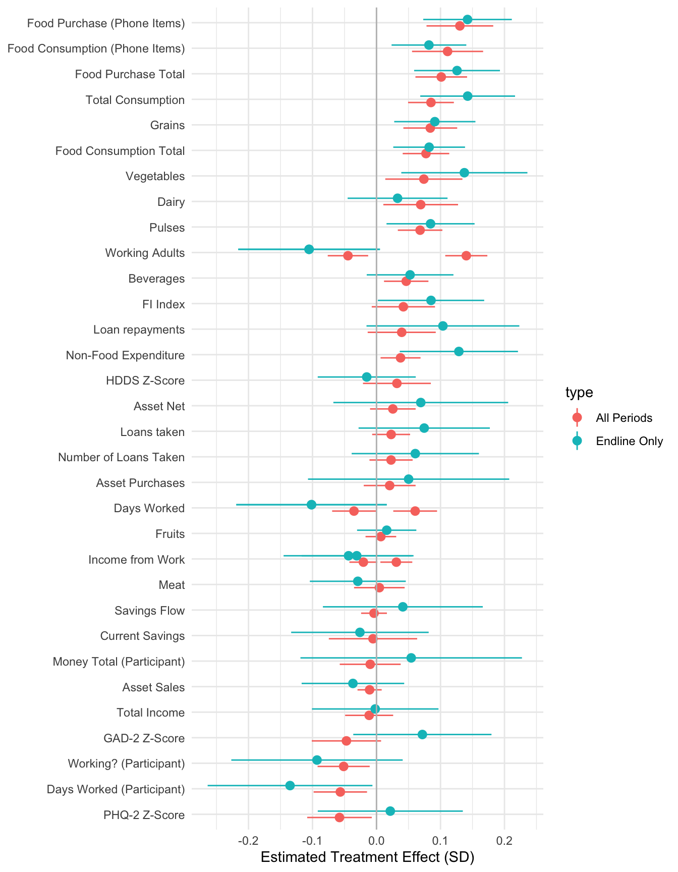
All regressions control for household size and wealth at census. They also include district_id, period, wave, enum_id, day_of_week and cohort fixed effects

1.1 Consumption and Purchases

1.1.1 Descriptive Graphs (mean)

Code
```{r}
#| warning: false
#| message: false
#| label: fig-total-consumption
#| fig-cap: "Total Consumption Over Time"
total_consumption <- ggplot(df, aes(x = period, y = total_consumption_99, color = treatment, group = treatment)) +
    geom_line(stat = "summary", fun = "mean") +
    labs(
        title = "All consumption",
        x = "Period",
        y = "Cedis (win. 99%)"
    ) +
    scale_color_discrete(
        name = "Treatment",
        labels = c("Control", "Stable", "Predictable", "Risky")
    )


non_food_expenditure <- ggplot(df, aes(x = period, y = expenditure_total_nonfood_99, color = treatment, group = treatment)) +
    geom_line(stat = "summary", fun = "mean") +
    labs(
        title = "Non-Food Consumption",
        x = "Period",
        y = "Cedis (win. 99%)"
    ) +
    scale_color_discrete(
        name = "Treatment",
        labels = c("Control", "Stable", "Predictable", "Risky")
    )

total_consumption / non_food_expenditure + plot_layout(guides = "collect") & theme(legend.justification = c("right", "top"))
```
Figure 1: Total Consumption Over Time

1.1.2 Period by Period Regression Coefficents

Code
```{r}
#| warning: false
#| message: false
total_consumption_reg_df <- df %>% generate_coeff_df("food_consumption_total_99")
total_consumption_reg_gp <- total_consumption_reg_df %>%
    effects_grapher("All Items")

total_consumption_reg_gp
```

1.1.3 Descriptive Graphs (mean)

Code
```{r}
#| warning: false
#| message: false
#| label: fig-food-consumption-detailed
#| fig-cap: "Food Consumption Over Time"
# Make ggplot showing how average food consumption changes over time by treatment
consumption <- ggplot(df, aes(x = period, y = food_consumption_total_99, color = treatment, group = treatment)) +
    geom_line(stat = "summary", fun = "mean") +
    labs(
        title = "Food Consumption - All Items",
        x = "Period",
        y = "Cedis (win. 99%)"
    ) +
    scale_color_discrete(
        name = "Treatment",
        labels = c("Control", "Stable", "Predictable", "Risky")
    ) +
    theme_minimal()

consumption_phone <- ggplot(df, aes(x = period, y = food_consumption_total_phone_99, color = treatment, group = treatment)) +
    geom_line(stat = "summary", fun = "mean") +
    labs(
        title = "Food Consumption - Phone Items",
        x = "Period",
        y = "Cedis (win. 99%)"
    ) +
    scale_color_discrete(
        name = "Treatment",
        labels = c("Control", "Stable", "Predictable", "Risky")
    ) +
    theme_minimal()


(consumption / consumption_phone) + plot_layout(guides = "collect") & theme(legend.justification = c("right", "top"))
```
Figure 2: Food Consumption Over Time

1.1.4 Period by Period Regression Coefficents

Code
```{r}
#| warning: false
#| message: false
cosnumption_reg_df <- df %>% generate_coeff_df("food_consumption_total_99")
consumption_reg_gp <- cosnumption_reg_df %>%
    effects_grapher("All Items")

consumption_phone_reg_gp <- df %>%
    generate_coeff_df("food_consumption_total_phone_99") %>%
    effects_grapher("Subset to Phone Items")

(consumption_reg_gp / consumption_phone_reg_gp) + plot_layout(guides = "collect", axes = "collect") + plot_annotation(title = "Treatment effect on food consumption (win 99%)")
```

Code
```{r}
#| label: fig-food-purchases-detailed
#| fig-cap: "Food Consumption Over Time"
#| warning: false
#| message: false
# Make ggplot showing how average food consumption changes over time by treatment
purchase <- ggplot(df, aes(x = period, y = food_purchase_total_99, color = treatment, group = treatment)) +
    geom_line(stat = "summary", fun = "mean") +
    labs(
        title = "Food Purchases - All Items",
        x = "Period",
        y = "Cedis (win. 99%)"
    ) +
    scale_color_discrete(
        name = "Treatment",
        labels = c("Control", "Stable", "Predictable", "Risky")
    ) +
    theme_minimal()

purchase_phone <- ggplot(df, aes(x = period, y = food_purchase_total_phone_99, color = treatment, group = treatment)) +
    geom_line(stat = "summary", fun = "mean") +
    labs(
        title = "Food Purchases - Phone Items",
        x = "Period",
        y = "Cedis (win. 99%)"
    ) +
    scale_color_discrete(
        name = "Treatment",
        labels = c("Control", "Stable", "Predictable", "Risky")
    ) +
    theme_minimal()

(purchase / purchase_phone) + plot_layout(guides = "collect") & theme(legend.justification = c("right", "top"))
```
Figure 3: Food Consumption Over Time

1.1.5 Period by Period Regression Coefficents

Code
```{r}
#| warning: false
#| message: false
purchase_reg_gp <- df %>%
    generate_coeff_df("food_purchase_total_99") %>%
    effects_grapher("All Items")

purchase_phone_reg_gp <- df %>%
    generate_coeff_df("food_purchase_total_phone_99") %>%
    effects_grapher("Subset to Phone Items")

(purchase_reg_gp / purchase_phone_reg_gp) + plot_layout(guides = "collect", axes = "collect") + plot_annotation(title = "Treatment effect on food purchases (win 99%)")
```

1.1.6 Food Consumption Regressions

Code
```{r}
#| label: tbl-consumption-main-results
#| tbl-cap: ""
# Create and output 1 table
makeTable(c(
    models[["total_consumption_99"]][1],
    models[["food_consumption_total_99"]][1],
    models[["food_purchase_total_99"]][1],
    models[["total_consumption_99"]][3],
    models[["food_consumption_total_99"]][3],
    models[["food_purchase_total_99"]][3]
))
```
Table 1
Total Consumption Food Consumption Total Food Purchase Total Total Consumption - Balanced Risky Food Consumption Total - Balanced Risky Food Purchase Total - Balanced Risky
Stable 66.156*** 36.084*** 52.976*** 66.911*** 37.123*** 54.081***
18.049 (30.762, 101.549) 13.660 (9.297, 62.871) 13.903 (25.713, 80.239) 18.079 (31.448, 102.375) 13.626 (10.395, 63.851) 13.932 (26.752, 81.410)
Predictable 63.801*** 57.188*** 48.864*** 62.095*** 56.723*** 47.959***
17.423 (29.634, 97.967) 14.013 (29.709, 84.667) 13.362 (22.662, 75.066) 17.385 (27.993, 96.197) 13.995 (29.270, 84.176) 13.339 (21.793, 74.125)
Risky 60.300*** 41.377*** 49.526***
14.373 (32.114, 88.486) 11.285 (19.248, 63.506) 10.953 (28.047, 71.005)
Risky (Balanced) 75.120*** 37.490** 56.735***
21.729 (32.497, 117.743) 16.074 (5.960, 69.020) 16.257 (24.845, 88.625)
Observations 14728 14728 14726 9426 9426 9425
Code
```{r}
#| label: tbl-consumption-treatment-timing
#| tbl-cap: ""
makeTable(c(
    models[["total_consumption_99"]][2],
    models[["food_consumption_total_99"]][2],
    models[["food_purchase_total_99"]][2]
))
```
Table 2
Total Consumption - Anticipation Effect Food Consumption Total - Anticipation Effect Food Purchase Total - Anticipation Effect
Stable 62.106*** 36.714** 53.277***
18.508 (25.812, 98.400) 14.374 (8.526, 64.902) 14.938 (23.983, 82.571)
Predictable Early 67.981*** 60.844*** 55.524***
22.586 (23.690, 112.273) 18.542 (24.481, 97.206) 17.740 (20.736, 90.311)
Predictable Late 54.188** 59.064*** 45.046***
21.524 (11.979, 96.396) 18.885 (22.030, 96.097) 17.097 (11.519, 78.573)
Risky Early 57.494*** 33.726** 48.887***
16.942 (24.271, 90.716) 13.924 (6.421, 61.031) 13.293 (22.818, 74.955)
Risky Late 55.777*** 57.187*** 55.363***
16.655 (23.117, 88.437) 13.729 (30.263, 84.110) 13.303 (29.275, 81.450)
Observations 10345 10345 10345
Code
```{r}
#| label: tbl-consumption-risky-splits
#| tbl-cap: ""
# Create and output 1 table
makeTable(c(
    models[["total_consumption_99"]][4],
    models[["food_consumption_total_99"]][4],
    models[["food_purchase_total_99"]][4]
))
```
Table 3
Total Consumption - Split Risky Food Consumption Total - Split Risky Food Purchase Total - Split Risky
Stable 66.156*** 35.915*** 52.930***
18.069 (30.717, 101.595) 13.649 (9.145, 62.685) 13.923 (25.622, 80.238)
Predictable 62.681*** 56.260*** 48.122***
17.393 (28.568, 96.793) 14.018 (28.767, 83.752) 13.348 (21.942, 74.303)
Risky Medium 74.196*** 36.448** 55.667***
21.634 (31.765, 116.628) 16.086 (4.899, 67.997) 16.206 (23.882, 87.451)
Risky High 37.321* 31.253* 28.011*
20.917 (−3.704, 78.345) 17.390 (−2.853, 65.359) 15.669 (−2.721, 58.742)
Risky Low 66.775*** 51.304*** 64.244***
23.865 (19.968, 113.582) 17.687 (16.614, 85.994) 18.491 (27.978, 100.510)
Observations 11492 11492 11490
Code
```{r}
#| label: tbl-consumption-income-interactions
#| tbl-cap: ""
# create and output 1 table
makeTable(c(
    models[["total_consumption_99"]][5],
    models[["food_consumption_total_99"]][5],
    models[["food_purchase_total_99"]][5],
    models[["total_consumption_99"]][6],
    models[["food_consumption_total_99"]][6],
    models[["food_purchase_total_99"]][6],
    models[["total_consumption_99"]][7],
    models[["food_consumption_total_99"]][7],
    models[["food_purchase_total_99"]][7]
))
```
Table 4
 Total Consumption - Income  Food Consumption Total - Income  Food Purchase Total - Income  Total Consumption - Income + Arm  Food Consumption Total - Income + Arm  Food Purchase Total - Income + Arm  Total Consumption - Income X Arm  Food Consumption Total - Income X Arm  Food Purchase Total - Income X Arm
Stable 66.957*** 37.433*** 55.823*** 60.436*** 29.269* 52.550***
18.636 (30.413, 103.502) 14.139 (9.706, 65.161) 14.308 (27.765, 83.880) 22.382 (16.544, 104.328) 17.705 (−5.451, 63.989) 17.884 (17.479, 87.621)
Predictable 64.588*** 58.514*** 51.663*** 43.975** 46.143*** 35.278**
18.149 (28.999, 100.178) 14.593 (29.897, 87.132) 13.818 (24.565, 78.761) 19.150 (6.422, 81.528) 15.441 (15.863, 76.424) 14.384 (7.071, 63.485)
Risky 61.087*** 42.702*** 52.322*** 68.911*** 47.628*** 58.435***
15.298 (31.088, 91.086) 11.846 (19.471, 65.933) 11.620 (29.535, 75.109) 15.577 (38.365, 99.457) 12.034 (24.029, 71.227) 11.807 (35.280, 81.589)
Study Income 0.170*** 0.111** 0.117** −0.009 −0.016 −0.034 −0.104 −0.075 −0.107*
0.064 (0.045, 0.296) 0.050 (0.013, 0.210) 0.048 (0.023, 0.211) 0.065 (−0.138, 0.119) 0.051 (−0.116, 0.084) 0.048 (−0.129, 0.061) 0.076 (−0.252, 0.045) 0.059 (−0.191, 0.041) 0.055 (−0.216, 0.001)
Stable × Study Income 0.171 0.155 0.112
0.207 (−0.235, 0.577) 0.156 (−0.150, 0.461) 0.168 (−0.217, 0.441)
Predictable × Study Income 0.344*** 0.209** 0.272***
0.125 (0.098, 0.589) 0.097 (0.018, 0.400) 0.090 (0.096, 0.448)
Observations 14728 14728 14726 14728 14728 14726 14728 14728 14726
Note

For risky arms that did not complete dropoff, we impute a medium draw for the regressions below

Code
```{r}
#| label: tbl-consumption-draw
#| tbl-cap: ""
# create and output 1 table
makeTable(c(
    models[["total_consumption_99"]][8],
    models[["food_consumption_total_99"]][8],
    models[["food_purchase_total_99"]][8],
    models[["total_consumption_99"]][9],
    models[["food_consumption_total_99"]][9],
    models[["food_purchase_total_99"]][9]
))
```
Table 5
 Total Consumption - Imputed Draw  Food Consumption Total - Imputed Draw  Food Purchase Total - Imputed Draw  Total Consumption - Imputed Draw with Lag  Food Consumption Total - Imputed Draw with Lag  Food Purchase Total - Imputed Draw with Lag
High Draw 63.895*** 53.607*** 48.588*** −75.554 −84.219 −62.671
18.553 (27.513, 100.277) 14.753 (24.676, 82.538) 14.311 (20.524, 76.651) 1.71627e+07 (−33656308.837, 33656157.728) 12343242.163 (−24205306.113, 24205137.675) 12346877.855 (−24212414.193, 24212288.851)
Medium Draw 71.271*** 45.104*** 54.393*** −83.770 −101.521 −75.475
16.830 (38.266, 104.275) 12.727 (20.147, 70.061) 12.977 (28.944, 79.842) 1.71627e+07 (−33656317.368, 33656149.827) 12343242.237 (−24205323.560, 24205120.519) 12346878.137 (−24212427.549, 24212276.600)
Low Draw 69.293*** 59.164*** 56.565*** −69.930 −78.114 −54.352
18.746 (32.531, 106.055) 15.038 (29.674, 88.654) 14.305 (28.512, 84.618) 1.71627e+07 (−33656302.577, 33656162.717) 12343241.710 (−24205299.119, 24205142.891) 12346877.630 (−24212405.432, 24212296.728)
High Draw previous period 132.147 130.601 101.991
1.71627e+07 (−33656102.561, 33656366.856) 12343242.294 (−24205091.550, 24205352.752) 12346878.420 (−24212250.639, 24212454.621)
Medium Draw previous period 157.192 148.692 132.661
1.71627e+07 (−33656076.999, 33656391.383) 12343242.410 (−24205073.685, 24205371.070) 12346878.321 (−24212219.775, 24212485.097)
Low Draw previous period 136.293 140.606 108.488
1.71627e+07 (−33656097.684, 33656370.270) 12343242.343 (−24205081.642, 24205362.853) 12346878.200 (−24212243.711, 24212460.686)
Observations 14728 14728 14726 14728 14728 14726
Note

Only treated participants that completed pickup are included in the regressions below.

Code
```{r}
#| label: tbl-consumption-imputed-draw
#| tbl-cap: ""
# create and output 1 table
makeTable(c(
    models[["total_consumption_99"]][10],
    models[["food_consumption_total_99"]][10],
    models[["food_purchase_total_99"]][10],
    models[["total_consumption_99"]][11],
    models[["food_consumption_total_99"]][11],
    models[["food_purchase_total_99"]][11]
))
```
Table 6
Total Consumption - Realized Draw Food Consumption Total - Realized Draw Food Purchase Total - Realized Draw Total Consumption - Realized Draw with Lag Food Consumption Total - Realized Draw with Lag Food Purchase Total - Realized Draw with Lag
High Draw 72.076*** 63.570*** 52.015*** 62.797*** 62.620*** 44.234***
19.382 (34.066, 110.086) 15.448 (33.275, 93.866) 14.870 (22.855, 81.175) 19.920 (23.733, 101.861) 15.578 (32.071, 93.170) 15.217 (14.393, 74.075)
Medium Draw 70.921*** 40.190*** 55.996*** 60.053*** 34.060** 45.106***
19.484 (32.713, 109.129) 14.530 (11.696, 68.684) 15.137 (26.313, 85.680) 19.598 (21.621, 98.485) 14.635 (5.360, 62.761) 15.167 (15.362, 74.850)
Low Draw 76.675*** 67.726*** 59.070*** 71.213*** 69.243*** 56.764***
19.660 (38.121, 115.229) 15.839 (36.665, 98.788) 14.929 (29.793, 88.348) 20.761 (30.499, 111.927) 16.687 (36.518, 101.968) 15.699 (25.977, 87.550)
High Draw previous period −5.328 −11.105 −7.220
9.818 (−24.581, 13.925) 7.535 (−25.881, 3.672) 6.887 (−20.727, 6.286)
Observations 12335 12335 12334 10755 10755 10754
Note

Only participants who completed all surveys are included in the regressions below.

Code
```{r}
#| label: tbl-consumption-balanced-panel
#| tbl-cap: ""
# create and output 1 table
makeTable(c(
    models[["total_consumption_99"]][12],
    models[["food_consumption_total_99"]][12],
    models[["food_purchase_total_99"]][12]
))
```
Table 7
Total Consumption - Balanced Panel Food Consumption Total - Balanced Panel Food Purchase Total - Balanced Panel
Stable 72.135*** 39.054** 53.786***
22.572 (27.859, 116.412) 17.048 (5.613, 72.494) 17.584 (19.295, 88.277)
Predictable 58.244*** 51.796*** 44.655***
21.683 (15.713, 100.776) 17.732 (17.013, 86.578) 16.922 (11.462, 77.849)
Risky 59.593*** 43.109*** 49.615***
18.125 (24.040, 95.147) 14.405 (14.852, 71.366) 14.165 (21.829, 77.401)
Observations 10493 10493 10492
Note

The regressions below include baseline (period 0) data.

Code
```{r}
#| label: tbl-consumption-baseline-included
#| tbl-cap: ""
makeTable(c(
    models[["total_consumption_99"]][16],
    models[["food_consumption_total_99"]][16],
    models[["food_purchase_total_99"]][16]
))
```
Table 8
 Total Consumption - Baseline Included  Food Consumption Total - Baseline Included  Food Purchase Total - Baseline Included
Stable 56.414*** 31.002** 45.468***
15.727 (25.573, 87.255) 12.167 (7.142, 54.862) 12.128 (21.685, 69.251)
Predictable 54.119*** 52.230*** 42.831***
15.210 (24.292, 83.946) 12.432 (27.851, 76.610) 11.703 (19.882, 65.780)
Risky 50.387*** 35.194*** 41.605***
12.534 (25.808, 74.966) 10.107 (15.374, 55.014) 9.562 (22.854, 60.356)
Observations 17000 17000 16998
Note

The regressions below exclude endline (period 6) data.

Code
```{r}
#| label: tbl-consumption-excluding-endline
#| tbl-cap: ""
makeTable(c(
    models[["total_consumption_99"]][17],
    models[["food_consumption_total_99"]][17],
    models[["food_purchase_total_99"]][17]
))
```
Table 9
Total Consumption - Excluding Endline Food Consumption Total - Excluding Endline Food Purchase Total - Excluding Endline
Stable 62.110*** 36.702** 53.273***
18.507 (25.818, 98.401) 14.376 (8.511, 64.893) 14.937 (23.982, 82.564)
Predictable 61.171*** 59.834*** 50.313***
17.821 (26.223, 96.118) 15.008 (30.404, 89.265) 14.094 (22.674, 77.951)
Risky 56.659*** 45.257*** 52.077***
14.769 (27.697, 85.621) 12.112 (21.505, 69.008) 11.701 (29.132, 75.023)
Observations 10345 10345 10345

1.2 Mental Health

Warning

The N for mental health outcomes is lower than for other outcomes. The cause for the lower observation count is due to 62 endline surveys that were conducted with a household member other than the participant. In these cases we did not ask for responses to the mental health questions.

1.2.1 Descriptive Graphs (mean)

Code
```{r}
#| label: fig-mental-health
#| fig-cap: "Mental Health Over Time"
#| warning: false
# Make ggplot showing how average food consumption changes over time by treatment
phq <- ggplot(df, aes(x = period, y = phq2_z, color = treatment, group = treatment)) +
    geom_line(stat = "summary", fun = "mean") +
    labs(
        title = "PHQ-2 Z-Score",
        x = "Period",
        y = "PHQ-2 Z-score",
    ) +
    scale_color_discrete(
        name = "Treatment",
        labels = c("Control", "Stable", "Predictable", "Risky")
    ) +
    theme_minimal()
gad <- ggplot(df, aes(x = period, y = gad2_z, color = treatment, group = treatment)) +
    geom_line(stat = "summary", fun = "mean") +
    labs(
        title = "GAD-2 Z-Score",
        x = "Period",
        y = "GAD-2 Z-score",
    ) +
    scale_color_discrete(
        name = "Treatment",
        labels = c("Control", "Stable", "Predictable", "Risky")
    ) +
    theme_minimal()

(gad / phq) + plot_layout(guides = "collect") & theme(legend.justification = c("right", "top"))
```
Figure 4: Mental Health Over Time

1.2.2 Period by Period Regression Coefficents

Code
```{r}
#| warning: false
#| message: false
gad_reg_gp <- df %>%
    generate_coeff_df("gad2_z") %>%
    effects_grapher("GAD-2 Z-Score")

phq_reg_gp <- df %>%
    generate_coeff_df("phq2_z") %>%
    effects_grapher("PHQ-2 Z-Score")

(gad_reg_gp / phq_reg_gp) + plot_layout(guides = "collect", axes = "collect") + plot_annotation(title = "Treatment effect on mental health")
```

1.2.3 Mental Health Regressions

Code
```{r}
#| label: tbl-mental-health-main
#| tbl-cap: ""
makeTable(c(
    models[["gad2_z"]][1],
    models[["phq2_z"]][1],
    models[["gad2_z"]][3],
    models[["phq2_z"]][3]
))
```
Table 10
 GAD-2 Z-Score  PHQ-2 Z-Score  GAD-2 Z-Score - Balanced Risky  PHQ-2 Z-Score - Balanced Risky
Stable −0.048 −0.055* −0.044 −0.053
0.034 (−0.115, 0.019) 0.033 (−0.119, 0.010) 0.034 (−0.111, 0.023) 0.033 (−0.118, 0.011)
Predictable −0.015 −0.019 −0.016 −0.022
0.035 (−0.083, 0.053) 0.032 (−0.082, 0.045) 0.035 (−0.084, 0.052) 0.032 (−0.086, 0.042)
Risky −0.059** −0.074***
0.029 (−0.116, −0.001) 0.027 (−0.127, −0.021)
Risky (Balanced) −0.033 −0.103***
0.041 (−0.112, 0.047) 0.036 (−0.174, −0.031)
Observations 14666 14666 9391 9391
Code
```{r}
#| label: tbl-mental-health-treatment-timing
#| tbl-cap: ""
makeTable(c(
    models[["gad2_z"]][2],
    models[["phq2_z"]][2]
))
```
Table 11
 GAD-2 Z-Score - Anticipation Effect  PHQ-2 Z-Score - Anticipation Effect
Stable −0.096*** −0.099***
0.037 (−0.170, −0.023) 0.035 (−0.167, −0.031)
Predictable Early −0.028 −0.063
0.043 (−0.112, 0.055) 0.040 (−0.142, 0.015)
Predictable Late −0.089* −0.048
0.046 (−0.180, 0.002) 0.045 (−0.136, 0.039)
Risky Early −0.092*** −0.107***
0.035 (−0.161, −0.024) 0.032 (−0.170, −0.043)
Risky Late −0.064* −0.084**
0.036 (−0.134, 0.005) 0.033 (−0.148, −0.020)
Observations 10345 10345
Code
```{r}
#| label: tbl-mental-health-risky-splits
#| tbl-cap: ""
makeTable(c(
    models[["gad2_z"]][4],
    models[["phq2_z"]][4]
))
```
Table 12
 GAD-2 Z-Score - Split Risky  PHQ-2 Z-Score - Split Risky
Stable −0.046 −0.055*
0.034 (−0.113, 0.021) 0.033 (−0.119, 0.009)
Predictable −0.017 −0.021
0.035 (−0.084, 0.051) 0.032 (−0.084, 0.043)
Risky Medium −0.034 −0.104***
0.041 (−0.114, 0.046) 0.037 (−0.175, −0.032)
Risky High −0.102** −0.067*
0.043 (−0.186, −0.018) 0.039 (−0.144, 0.010)
Risky Low −0.005 −0.039
0.049 (−0.102, 0.091) 0.046 (−0.129, 0.051)
Observations 11438 11438
Code
```{r}
#| label: tbl-mental-health-income-interactions
#| tbl-cap: ""
makeTable(c(
    models[["gad2_z"]][5],
    models[["phq2_z"]][5],
    models[["gad2_z"]][6],
    models[["phq2_z"]][6],
    models[["gad2_z"]][7],
    models[["phq2_z"]][7]
))
```
Table 13
 GAD-2 Z-Score - Income  PHQ-2 Z-Score - Income  GAD-2 Z-Score - Income + Arm  PHQ-2 Z-Score - Income + Arm  GAD-2 Z-Score - Income X Arm  PHQ-2 Z-Score - Income X Arm
Stable −0.015 −0.029 0.003 −0.031
0.036 (−0.085, 0.055) 0.034 (−0.096, 0.039) 0.052 (−0.098, 0.105) 0.050 (−0.130, 0.067)
Predictable 0.018 0.007 0.013 −0.005
0.036 (−0.053, 0.089) 0.034 (−0.060, 0.074) 0.039 (−0.063, 0.089) 0.038 (−0.080, 0.069)
Risky −0.025 −0.048* −0.025 −0.044
0.031 (−0.086, 0.035) 0.029 (−0.105, 0.009) 0.032 (−0.087, 0.038) 0.029 (−0.101, 0.014)
Study Income −0.000*** −0.000*** −0.000*** −0.000** −0.000*** −0.000***
0.000 (−0.001, −0.000) 0.000 (−0.001, −0.000) 0.000 (−0.001, −0.000) 0.000 (−0.001, −0.000) 0.000 (−0.001, −0.000) 0.000 (−0.001, −0.000)
Stable × Study Income −0.000 0.000
0.000 (−0.001, 0.001) 0.000 (−0.001, 0.001)
Predictable × Study Income 0.000 0.000
0.000 (−0.000, 0.001) 0.000 (−0.000, 0.001)
Observations 14666 14666 14666 14666 14666 14666
Note

For risky arms that did not complete dropoff, we impute a medium draw for the regressions below

Code
```{r}
#| label: tbl-mental-health-draw
#| tbl-cap: ""
makeTable(c(
    models[["gad2_z"]][8],
    models[["phq2_z"]][8],
    models[["gad2_z"]][9],
    models[["phq2_z"]][9]
))
```
Table 14
 GAD-2 Z-Score - Imputed Draw  PHQ-2 Z-Score - Imputed Draw  GAD-2 Z-Score - Imputed Draw with Lag  PHQ-2 Z-Score - Imputed Draw with Lag
High Draw −0.062* −0.064* 0.090 −0.448
0.037 (−0.134, 0.011) 0.034 (−0.131, 0.003) 11908.501 (−23352.618, 23352.797) 10900.383 (−21376.223, 21375.327)
Medium Draw −0.046 −0.043 0.104 −0.412
0.033 (−0.110, 0.018) 0.031 (−0.104, 0.018) 11908.501 (−23352.602, 23352.810) 10900.382 (−21376.185, 21375.362)
Low Draw −0.014 −0.039 0.138 −0.423
0.037 (−0.086, 0.059) 0.034 (−0.106, 0.028) 11908.501 (−23352.569, 23352.846) 10900.383 (−21376.199, 21375.353)
High Draw previous period −0.154 0.381
11908.498 (−23352.855, 23352.548) 10900.380 (−21375.388, 21376.151)
Medium Draw previous period −0.146 0.364
11908.499 (−23352.848, 23352.556) 10900.381 (−21375.407, 21376.135)
Low Draw previous period −0.142 0.391
11908.499 (−23352.844, 23352.560) 10900.380 (−21375.379, 21376.160)
Observations 14666 14666 14666 14666
Note

Only treated participants that completed pickup are included in the regressions below.

Code
```{r}
#| label: tbl-mental-health-imputed-draw
#| tbl-cap: ""
makeTable(c(
    models[["gad2_z"]][10],
    models[["phq2_z"]][10],
    models[["gad2_z"]][11],
    models[["phq2_z"]][11]
))
```
Table 15
 GAD-2 Z-Score - Realized Draw  PHQ-2 Z-Score - Realized Draw  GAD-2 Z-Score - Realized Draw with Lag  PHQ-2 Z-Score - Realized Draw with Lag
High Draw −0.052 −0.048 0.735 −0.349
0.038 (−0.127, 0.023) 0.036 (−0.117, 0.022) 22272.341 (−43676.613, 43678.083) 20548.332 (−40296.815, 40296.117)
Medium Draw −0.060 −0.064* −0.055 −0.070*
0.037 (−0.132, 0.012) 0.035 (−0.133, 0.004) 0.038 (−0.129, 0.018) 0.036 (−0.140, 0.001)
Low Draw −0.003 −0.020 0.777 −0.329
0.038 (−0.078, 0.073) 0.036 (−0.090, 0.050) 22272.341 (−43676.571, 43678.126) 20548.333 (−40296.797, 40296.139)
High Draw previous period −0.802 0.295
22272.338 (−43678.145, 43676.540) 20548.329 (−40296.166, 40296.756)
Low Draw previous period −0.793 0.294
22272.338 (−43678.136, 43676.550) 20548.329 (−40296.167, 40296.755)
Observations 12298 12298 10719 10719
Note

Only participants who completed all surveys are included in the regressions below.

Code
```{r}
#| label: tbl-mental-health-balanced-panel
#| tbl-cap: ""
makeTable(c(
    models[["gad2_z"]][12],
    models[["phq2_z"]][12]
))
```
Table 16
 GAD-2 Z-Score - Balanced Panel  PHQ-2 Z-Score - Balanced Panel
Stable −0.092** −0.107***
0.042 (−0.175, −0.008) 0.041 (−0.186, −0.027)
Predictable −0.024 −0.059
0.043 (−0.109, 0.061) 0.041 (−0.139, 0.021)
Risky −0.089** −0.116***
0.037 (−0.161, −0.016) 0.035 (−0.184, −0.048)
Observations 10469 10469
Note

The regressions below include baseline (period 0) data.

Code
```{r}
#| label: tbl-mental-health-baseline-included
#| tbl-cap: ""
makeTable(c(
    models[["gad2_z"]][16],
    models[["phq2_z"]][16]
))
```
Table 17
 GAD-2 Z-Score - Baseline Included  PHQ-2 Z-Score - Baseline Included
Stable −0.046 −0.049*
0.030 (−0.105, 0.013) 0.029 (−0.106, 0.007)
Predictable −0.008 −0.012
0.030 (−0.068, 0.051) 0.028 (−0.068, 0.044)
Risky −0.051** −0.065***
0.025 (−0.101, −0.001) 0.024 (−0.111, −0.018)
Observations 16938 16938
Note

The regressions below exclude endline (period 6) data.

Code
```{r}
#| label: tbl-mental-health-excluding-endline
#| tbl-cap: ""
makeTable(c(
    models[["gad2_z"]][17],
    models[["phq2_z"]][17]
))
```
Table 18
 GAD-2 Z-Score - Excluding Endline  PHQ-2 Z-Score - Excluding Endline
Stable −0.096*** −0.099***
0.037 (−0.170, −0.023) 0.035 (−0.167, −0.032)
Predictable −0.059 −0.056
0.037 (−0.131, 0.014) 0.035 (−0.124, 0.012)
Risky −0.079** −0.096***
0.032 (−0.141, −0.016) 0.029 (−0.153, −0.039)
Observations 10345 10345

1.3 Income and Days Worked

Note

The variables included in total income are:

  • Work Income
  • Income from crop or ag. product sales
  • Income from “other sources” (remittances and sales of goods mostly)
Tip

During period 4, we made a change in the survey to account for the fact the participants were including study income in their reported income.

1.3.1 Descriptive Graphs (mean)

Code
```{r}
#| label: fig-money-earned
#| fig-cap: "Work Outcomes Over Time"
#| warning: false

total_income_plot <- ggplot(df, aes(x = period, y = total_income_99, color = treatment, group = treatment)) +
    geom_line(stat = "summary", fun = "mean") +
    labs(
        title = "Total Income (Household)",
        x = "Period",
        y = "Cedis"
    ) +
    scale_color_discrete(
        name = "Treatment",
        labels = c("Control", "Stable", "Predictable", "Risky")
    ) +
    theme_minimal()

working_adults_plot <- ggplot(df, aes(x = period, y = working_adults_corrected, color = treatment, group = treatment)) +
    geom_line(stat = "summary", fun = "mean") +
    labs(
        title = "Working Adults (Household)",
        x = "Period",
        y = "Count"
    ) +
    scale_color_discrete(
        name = "Treatment",
        labels = c("Control", "Stable", "Predictable", "Risky")
    ) +
    theme_minimal()

days_worked_corrected_plot <- ggplot(df, aes(x = period, y = days_worked_corrected, color = treatment, group = treatment)) +
    geom_line(stat = "summary", fun = "mean") +
    labs(
        title = "Days Worked (Household)",
        x = "Period",
        y = "Days"
    ) +
    scale_color_discrete(
        name = "Treatment",
        labels = c("Control", "Stable", "Predictable", "Risky")
    ) +
    theme_minimal()

money_work_plot <- ggplot(df, aes(x = period, y = money_work_corrected_99, color = treatment, group = treatment)) +
    geom_line(stat = "summary", fun = "mean") +
    labs(
        title = "Work Income (Household)",
        x = "Period",
        y = "Cedis"
    ) +
    scale_color_discrete(
        name = "Treatment",
        labels = c("Control", "Stable", "Predictable", "Risky")
    ) +
    theme_minimal()

((total_income_plot + working_adults_plot) / days_worked_corrected_plot / money_work_plot) + plot_layout(guides = "collect") & theme(legend.justification = c("right", "top"))
```
Figure 5: Work Outcomes Over Time

1.3.2 Period by Period Regression Coefficents

Code
```{r}
#| warning: false
#| message: false
total_income_reg_gp <- df %>%
    generate_coeff_df("total_income_99") %>%
    effects_grapher("Total Income (Cedis)")

working_adults_reg_gp <- df %>%
    generate_coeff_df("working_adults_corrected") %>%
    effects_grapher("Working Adults")

days_worked_corrected_reg_gp <- df %>%
    generate_coeff_df("days_worked_corrected") %>%
    effects_grapher("Days Worked")

money_work_reg_gp <- df %>%
    generate_coeff_df("money_work_corrected_99") %>%
    effects_grapher("Work Income (Cedis)")

((total_income_reg_gp + working_adults_reg_gp) / days_worked_corrected_reg_gp / money_work_reg_gp) + plot_layout(guides = "collect", axes = "collect") + plot_annotation(title = "Treatment effect on household work")
```

1.3.3 Descriptive Graphs (mean)

Code
```{r}
#| label: fig-money-earned-p
#| fig-cap: "Work Outcomes Over Time"
#| warning: false

working_adults_plot <- ggplot(df, aes(x = period, y = work_engaged_p_corrected, color = treatment, group = treatment)) +
    geom_line(stat = "summary", fun = "mean") +
    labs(
        title = "Working? (participant)",
        x = "Period",
        y = "Count"
    ) +
    scale_color_discrete(
        name = "Treatment",
        labels = c("Control", "Stable", "Predictable", "Risky")
    ) +
    theme_minimal()

days_worked_corrected_plot <- ggplot(df, aes(x = period, y = days_worked_p_corrected, color = treatment, group = treatment)) +
    geom_line(stat = "summary", fun = "mean") +
    labs(
        title = "Days Worked (Participant)",
        x = "Period",
        y = "Days"
    ) +
    scale_color_discrete(
        name = "Treatment",
        labels = c("Control", "Stable", "Predictable", "Risky")
    ) +
    theme_minimal()

money_work_plot <- ggplot(df, aes(x = period, y = money_work_p_corrected_99, color = treatment, group = treatment)) +
    geom_line(stat = "summary", fun = "mean") +
    labs(
        title = "Work Income (Participant)",
        x = "Period",
        y = "Cedis"
    ) +
    scale_color_discrete(
        name = "Treatment",
        labels = c("Control", "Stable", "Predictable", "Risky")
    ) +
    theme_minimal()

(working_adults_plot / days_worked_corrected_plot / money_work_plot) + plot_layout(guides = "collect") & theme(legend.justification = c("right", "top"))
```
Figure 6: Work Outcomes Over Time

1.3.4 Period by Period Regression Coefficents

Code
```{r}
#| warning: false
#| message: false
#| label: fig-money-earned-p-reg
working_adults_reg_gp <- df %>%
    generate_coeff_df("work_engaged_p_corrected") %>%
    effects_grapher("Working?")

days_worked_corrected_reg_gp <- df %>%
    generate_coeff_df("days_worked_p_corrected") %>%
    effects_grapher("Days Worked")

money_work_reg_gp <- df %>%
    generate_coeff_df("money_earn_p_corrected") %>%
    effects_grapher("Work Income")

(working_adults_reg_gp / days_worked_corrected_reg_gp / money_work_reg_gp) + plot_layout(guides = "collect", axes = "collect") + plot_annotation(title = "Treatment effect on participant outside work")
```
Figure 7

1.3.5 Work Regressions

Code
```{r}
#| label: tbl-money-earned-main
#| tbl-cap: ""
makeTable(c(
    models[["working_adults_corrected"]][1], models[["days_worked_corrected"]][1], models[["money_work_corrected_99"]][1], models[["total_income_99"]][1],
    models[["working_adults_corrected"]][3], models[["days_worked_corrected"]][3], models[["money_work_corrected_99"]][3], models[["total_income_99"]][3],
    models[["days_worked_p_corrected"]][1], models[["money_earn_p_corrected"]][1], models[["work_engaged_p_corrected"]][1],
    models[["days_worked_p_corrected"]][3], models[["money_earn_p_corrected"]][3], models[["work_engaged_p_corrected"]][3]
))
```
Table 19
Working Adults Days Worked  Income from Work  Total Income Working Adults - Balanced Risky Days Worked - Balanced Risky  Income from Work - Balanced Risky  Total Income - Balanced Risky Days Worked (Participant) Money Total (Participant) Working? (Participant) Days Worked (Participant) - Balanced Risky Money Total (Participant) - Balanced Risky Working? (Participant) - Balanced Risky
Stable −0.060*** −0.325** −8.664** −23.131* −0.059*** −0.318** −8.393** −22.408 −0.153*** −1.265 −0.022*** −0.149*** −1.191 −0.022***
0.018 (−0.096, −0.024) 0.130 (−0.580, −0.070) 3.822 (−16.159, −1.169) 14.026 (−50.637, 4.374) 0.018 (−0.096, −0.023) 0.131 (−0.575, −0.061) 3.838 (−15.922, −0.865) 14.125 (−50.115, 5.299) 0.050 (−0.252, −0.055) 2.387 (−5.947, 3.417) 0.008 (−0.038, −0.007) 0.051 (−0.248, −0.049) 2.363 (−5.826, 3.444) 0.008 (−0.038, −0.006)
Predictable −0.045** −0.162 −3.795 17.854 −0.046** −0.161 −3.790 19.156 −0.100* −0.392 −0.018** −0.100* −0.055 −0.019**
0.018 (−0.081, −0.010) 0.129 (−0.416, 0.091) 3.859 (−11.363, 3.772) 15.322 (−12.193, 47.901) 0.018 (−0.082, −0.011) 0.130 (−0.415, 0.094) 3.865 (−11.372, 3.792) 15.378 (−11.010, 49.322) 0.051 (−0.201, 0.001) 2.434 (−5.164, 4.381) 0.008 (−0.034, −0.003) 0.052 (−0.201, 0.001) 2.405 (−4.772, 4.662) 0.008 (−0.034, −0.003)
Risky −0.030** −0.172 −4.731 −9.895 −0.102** −0.504 −0.014*
0.015 (−0.060, −0.000) 0.106 (−0.379, 0.035) 3.090 (−10.790, 1.328) 12.010 (−33.446, 13.656) 0.045 (−0.190, −0.015) 1.673 (−3.784, 2.776) 0.007 (−0.027, 0.000)
Risky (Balanced) −0.058*** −0.285** −10.933*** −15.047 −0.150*** −4.326** −0.024***
0.019 (−0.096, −0.021) 0.134 (−0.548, −0.021) 3.768 (−18.324, −3.542) 15.384 (−45.224, 15.130) 0.055 (−0.258, −0.042) 1.681 (−7.623, −1.028) 0.009 (−0.042, −0.007)
Observations 14728 14728 14728 14728 9426 9426 9426 9426 14728 14728 14728 9426 9426 9426
Code
```{r}
#| label: tbl-money-earned-treatment-timing
#| tbl-cap: ""
makeTable(c(
    models[["working_adults_corrected"]][2], models[["days_worked_corrected"]][2], models[["money_work_corrected_99"]][2], models[["total_income_99"]][2],
    models[["days_worked_p_corrected"]][2], models[["money_earn_p_corrected"]][2], models[["work_engaged_p_corrected"]][2]
))
```
Table 20
Working Adults - Anticipation Effect Days Worked - Anticipation Effect  Income from Work - Anticipation Effect  Total Income - Anticipation Effect Days Worked (Participant) - Anticipation Effect Money Total (Participant) - Anticipation Effect Working? (Participant) - Anticipation Effect
Stable −0.052*** −0.248* −8.615** −26.852* −0.127** −2.151 −0.022**
0.020 (−0.091, −0.014) 0.148 (−0.539, 0.043) 3.657 (−15.787, −1.444) 14.387 (−55.065, 1.360) 0.058 (−0.241, −0.014) 2.681 (−7.409, 3.106) 0.009 (−0.039, −0.004)
Predictable Early −0.031 −0.070 −4.240 10.894 −0.078 −4.239** −0.016
0.024 (−0.078, 0.016) 0.184 (−0.431, 0.290) 4.272 (−12.618, 4.137) 19.630 (−27.601, 49.389) 0.072 (−0.220, 0.063) 2.147 (−8.449, −0.028) 0.011 (−0.038, 0.005)
Predictable Late −0.034 −0.057 −4.695 18.397 −0.103 1.355 −0.018*
0.023 (−0.080, 0.013) 0.178 (−0.406, 0.292) 4.915 (−14.334, 4.943) 19.994 (−20.812, 57.605) 0.067 (−0.234, 0.027) 5.150 (−8.745, 11.455) 0.010 (−0.038, 0.002)
Risky Early −0.030 −0.160 −6.775** −13.039 −0.080 −2.223 −0.011
0.019 (−0.067, 0.007) 0.135 (−0.424, 0.104) 3.312 (−13.270, −0.280) 14.259 (−41.000, 14.922) 0.055 (−0.188, 0.029) 1.980 (−6.106, 1.660) 0.009 (−0.028, 0.006)
Risky Late −0.026 −0.069 −5.072 −10.274 −0.095* −2.206 −0.017*
0.019 (−0.063, 0.011) 0.141 (−0.345, 0.207) 3.414 (−11.767, 1.622) 14.463 (−38.635, 18.088) 0.057 (−0.206, 0.017) 2.106 (−6.335, 1.923) 0.009 (−0.033, 0.000)
Observations 10345 10345 10345 10345 10345 10345 10345
Code
```{r}
#| label: tbl-money-earned-risky-splits
#| tbl-cap: ""
makeTable(c(
    models[["working_adults_corrected"]][4], models[["days_worked_corrected"]][4], models[["money_work_corrected_99"]][4], models[["total_income_99"]][4],
    models[["days_worked_p_corrected"]][4], models[["money_earn_p_corrected"]][4], models[["work_engaged_p_corrected"]][4]
))
```
Table 21
Working Adults - Split Risky Days Worked - Split Risky  Income from Work - Split Risky  Total Income - Split Risky Days Worked (Participant) - Split Risky Money Total (Participant) - Split Risky Working? (Participant) - Split Risky
Stable −0.060*** −0.328** −8.579** −23.133 −0.151*** −1.133 −0.022***
0.018 (−0.096, −0.024) 0.130 (−0.584, −0.072) 3.829 (−16.088, −1.069) 14.075 (−50.738, 4.473) 0.050 (−0.250, −0.053) 2.382 (−5.805, 3.538) 0.008 (−0.038, −0.006)
Predictable −0.046** −0.165 −3.888 18.536 −0.101** −0.274 −0.018**
0.018 (−0.081, −0.010) 0.129 (−0.419, 0.088) 3.866 (−11.470, 3.695) 15.345 (−11.560, 48.633) 0.051 (−0.202, −0.000) 2.434 (−5.049, 4.500) 0.008 (−0.034, −0.003)
Risky Medium −0.059*** −0.297** −10.643*** −14.443 −0.156*** −4.391** −0.025***
0.019 (−0.097, −0.022) 0.134 (−0.560, −0.034) 3.776 (−18.050, −3.237) 15.316 (−44.482, 15.597) 0.055 (−0.264, −0.048) 1.717 (−7.757, −1.024) 0.009 (−0.042, −0.007)
Risky High −0.029 −0.233 1.635 −7.483 −0.061 5.407 −0.006
0.022 (−0.073, 0.015) 0.148 (−0.524, 0.057) 5.047 (−8.263, 11.534) 18.567 (−43.898, 28.932) 0.069 (−0.196, 0.074) 3.727 (−1.904, 12.718) 0.010 (−0.026, 0.015)
Risky Low 0.013 −0.092 2.841 −5.980 −0.143** −2.189 −0.008
0.028 (−0.042, 0.067) 0.186 (−0.456, 0.272) 5.943 (−8.815, 14.497) 20.150 (−45.501, 33.541) 0.066 (−0.273, −0.013) 2.329 (−6.757, 2.380) 0.011 (−0.029, 0.014)
Observations 11492 11492 11492 11492 11492 11492 11492
Code
```{r}
#| label: tbl-money-earned-income-interactions
#| tbl-cap: ""
makeTable(c(
    models[["working_adults_corrected"]][5], models[["days_worked_corrected"]][5], models[["money_work_corrected_99"]][5], models[["total_income_99"]][5],
    models[["working_adults_corrected"]][6], models[["days_worked_corrected"]][6], models[["money_work_corrected_99"]][6], models[["total_income_99"]][6],
    models[["working_adults_corrected"]][7], models[["days_worked_corrected"]][7], models[["money_work_corrected_99"]][7], models[["total_income_99"]][7],
    models[["days_worked_p_corrected"]][5], models[["money_earn_p_corrected"]][5], models[["work_engaged_p_corrected"]][5],
    models[["days_worked_p_corrected"]][6], models[["money_earn_p_corrected"]][6], models[["work_engaged_p_corrected"]][6],
    models[["days_worked_p_corrected"]][7], models[["money_earn_p_corrected"]][7], models[["work_engaged_p_corrected"]][7]
))
```
Table 22
 Working Adults - Income  Days Worked - Income  Income from Work - Income  Total Income - Income  Working Adults - Income + Arm  Days Worked - Income + Arm  Income from Work - Income + Arm  Total Income - Income + Arm  Working Adults - Income X Arm  Days Worked - Income X Arm  Income from Work - Income X Arm  Total Income - Income X Arm  Days Worked (Participant) - Income  Money Total (Participant) - Income  Working? (Participant) - Income  Days Worked (Participant) - Income + Arm  Money Total (Participant) - Income + Arm  Working? (Participant) - Income + Arm  Days Worked (Participant) - Income X Arm  Money Total (Participant) - Income X Arm  Working? (Participant) - Income X Arm
Stable −0.048** −0.245* −8.062** −17.122 −0.053** −0.330** −4.754 −12.649 −0.119** −0.126 −0.018** −0.092 2.647 −0.018**
0.019 (−0.086, −0.009) 0.137 (−0.513, 0.023) 4.077 (−16.056, −0.067) 14.686 (−45.922, 11.678) 0.021 (−0.094, −0.011) 0.144 (−0.612, −0.047) 4.647 (−13.867, 4.359) 21.481 (−54.774, 29.476) 0.053 (−0.223, −0.015) 2.675 (−5.371, 5.119) 0.008 (−0.034, −0.001) 0.060 (−0.210, 0.026) 3.944 (−5.088, 10.382) 0.009 (−0.035, −0.000)
Predictable −0.033* −0.084 −3.202 23.762 −0.038* −0.138 −6.657 11.688 −0.066 0.728 −0.014 −0.066 −0.623 −0.014
0.019 (−0.071, 0.005) 0.138 (−0.354, 0.186) 4.029 (−11.103, 4.699) 15.684 (−6.995, 54.519) 0.021 (−0.080, 0.004) 0.156 (−0.444, 0.168) 4.058 (−14.614, 1.300) 17.014 (−21.677, 45.052) 0.054 (−0.172, 0.040) 2.518 (−4.210, 5.665) 0.008 (−0.030, 0.003) 0.059 (−0.182, 0.050) 2.268 (−5.070, 3.824) 0.009 (−0.032, 0.004)
Risky −0.018 −0.093 −4.139 −3.993 −0.016 −0.069 −3.069 0.135 −0.068 0.614 −0.009 −0.070 0.952 −0.009
0.017 (−0.051, 0.015) 0.115 (−0.318, 0.131) 3.420 (−10.846, 2.569) 13.034 (−29.554, 21.567) 0.017 (−0.050, 0.018) 0.117 (−0.299, 0.161) 3.546 (−10.023, 3.886) 13.439 (−26.220, 26.490) 0.048 (−0.163, 0.026) 2.073 (−3.450, 4.679) 0.008 (−0.024, 0.006) 0.050 (−0.167, 0.027) 2.214 (−3.389, 5.293) 0.008 (−0.024, 0.007)
Study Income −0.000*** −0.001** −0.021 −0.075 −0.000 −0.001 −0.007 −0.071 −0.000 −0.001* −0.020 −0.121* −0.001*** −0.012 −0.000** −0.000 −0.013 −0.000 −0.000 −0.018 −0.000
0.000 (−0.000, −0.000) 0.001 (−0.002, −0.000) 0.017 (−0.055, 0.013) 0.056 (−0.184, 0.034) 0.000 (−0.000, 0.000) 0.001 (−0.002, 0.000) 0.019 (−0.045, 0.031) 0.058 (−0.185, 0.043) 0.000 (−0.000, 0.000) 0.001 (−0.003, 0.000) 0.023 (−0.064, 0.024) 0.066 (−0.251, 0.009) 0.000 (−0.001, −0.000) 0.010 (−0.031, 0.007) 0.000 (−0.000, −0.000) 0.000 (−0.001, 0.000) 0.012 (−0.037, 0.010) 0.000 (−0.000, 0.000) 0.000 (−0.001, 0.000) 0.014 (−0.045, 0.010) 0.000 (−0.000, 0.000)
Stable × Study Income 0.000 0.001 −0.026 −0.003 −0.000 −0.029 0.000
0.000 (−0.000, 0.001) 0.002 (−0.002, 0.005) 0.043 (−0.110, 0.058) 0.186 (−0.368, 0.362) 0.001 (−0.002, 0.001) 0.029 (−0.086, 0.029) 0.000 (−0.000, 0.000)
Predictable × Study Income 0.000 0.001 0.055 0.196 −0.000 0.020 0.000
0.000 (−0.000, 0.000) 0.001 (−0.002, 0.004) 0.035 (−0.014, 0.124) 0.122 (−0.043, 0.435) 0.000 (−0.001, 0.001) 0.019 (−0.016, 0.057) 0.000 (−0.000, 0.000)
Observations 14728 14728 14728 14728 14728 14728 14728 14728 14728 14728 14728 14728 14728 14728 14728 14728 14728 14728 14728 14728 14728
Note

For risky arms that did not complete dropoff, we impute a medium draw for the regressions below

Code
```{r}
#| label: tbl-money-earned-draw
#| tbl-cap: ""
makeTable(c(
    models[["working_adults_corrected"]][8], models[["days_worked_corrected"]][8], models[["money_work_corrected_99"]][8], models[["total_income_99"]][8],
    models[["working_adults_corrected"]][9], models[["days_worked_corrected"]][9], models[["money_work_corrected_99"]][9], models[["total_income_99"]][9],
    models[["days_worked_p_corrected"]][8], models[["money_earn_p_corrected"]][8], models[["work_engaged_p_corrected"]][8],
    models[["days_worked_p_corrected"]][9], models[["money_earn_p_corrected"]][9], models[["work_engaged_p_corrected"]][9]
))
```
Table 23
 Working Adults - Imputed Draw  Days Worked - Imputed Draw  Income from Work - Imputed Draw  Total Income - Imputed Draw  Working Adults - Imputed Draw with Lag  Days Worked - Imputed Draw with Lag  Income from Work - Imputed Draw with Lag  Total Income - Imputed Draw with Lag  Days Worked (Participant) - Imputed Draw  Money Total (Participant) - Imputed Draw  Working? (Participant) - Imputed Draw  Days Worked (Participant) - Imputed Draw with Lag  Money Total (Participant) - Imputed Draw with Lag  Working? (Participant) - Imputed Draw with Lag
High Draw −0.069*** −0.295* −7.070 2.536 1.560 1.416 6.407 −33.249 −0.160** −2.971 −0.028*** 0.690 4.457 0.709
0.021 (−0.111, −0.027) 0.153 (−0.595, 0.005) 4.642 (−16.172, 2.033) 16.408 (−29.640, 34.712) 16354.480 (−32069.740, 32072.860) 116608.636 (−228669.291, 228672.124) 4154909.968 (−8147813.785, 8147826.599) 17702373.048 (−34714564.651, 34714498.152) 0.063 (−0.283, −0.037) 3.050 (−8.951, 3.010) 0.010 (−0.046, −0.009) 48323.900 (−94762.962, 94764.343) 2611474.681 (−5121123.631, 5121132.545) 7921.702 (−15533.829, 15535.246)
Medium Draw −0.055*** −0.260** −5.976 −9.843 1.574 1.456 6.587 −43.979 −0.124** 0.535 −0.020** 0.769 8.146 0.725
0.018 (−0.090, −0.020) 0.127 (−0.508, −0.011) 3.778 (−13.384, 1.432) 13.319 (−35.961, 16.276) 16354.479 (−32069.724, 32072.871) 116608.628 (−228669.235, 228672.147) 4154910.386 (−8147814.425, 8147827.599) 17702373.129 (−34714575.540, 34714487.582) 0.050 (−0.222, −0.026) 2.405 (−4.181, 5.251) 0.008 (−0.035, −0.005) 48323.898 (−94762.880, 94764.418) 2611474.175 (−5121118.949, 5121135.241) 7921.702 (−15533.812, 15535.261)
Low Draw −0.056*** −0.238 −8.464* 9.975 1.574 1.480 5.254 −25.842 −0.155** −3.647 −0.024** 0.695 3.804 0.712
0.022 (−0.098, −0.013) 0.153 (−0.537, 0.061) 4.584 (−17.452, 0.525) 16.364 (−22.115, 42.064) 16354.481 (−32069.727, 32072.875) 116608.643 (−228669.241, 228672.201) 4154910.209 (−8147815.409, 8147825.918) 17702373.118 (−34714557.382, 34714505.697) 0.062 (−0.277, −0.033) 3.161 (−9.846, 2.551) 0.010 (−0.043, −0.006) 48323.901 (−94762.961, 94764.351) 2611474.805 (−5121124.527, 5121132.135) 7921.702 (−15533.825, 15535.250)
High Draw previous period −1.634 −1.737 −15.806 37.462 −0.832 −7.533 −0.736
16354.481 (−32072.936, 32069.668) 116608.643 (−228672.457, 228668.983) 4154909.730 (−8147835.531, 8147803.918) 17702370.761 (−34714489.455, 34714564.379) 48323.895 (−94764.476, 94762.812) 2611474.819 (−5121135.892, 5121120.825) 7921.702 (−15535.273, 15533.801)
Medium Draw previous period −1.624 −1.680 −12.173 34.798 −0.900 −7.577 −0.746
16354.480 (−32072.923, 32069.675) 116608.628 (−228672.371, 228669.011) 4154910.092 (−8147832.608, 8147808.262) 17702371.874 (−34714494.303, 34714563.899) 48323.894 (−94764.542, 94762.743) 2611474.700 (−5121135.701, 5121120.547) 7921.702 (−15535.283, 15533.790)
Low Draw previous period −1.615 −1.616 −11.385 36.990 −0.841 −7.102 −0.733
16354.481 (−32072.916, 32069.687) 116608.641 (−228672.333, 228669.101) 4154909.775 (−8147831.198, 8147808.428) 17702371.959 (−34714492.276, 34714566.256) 48323.896 (−94764.486, 94762.804) 2611474.893 (−5121135.605, 5121121.402) 7921.702 (−15535.270, 15533.804)
Observations 14728 14728 14728 14728 14728 14728 14728 14728 14728 14728 14728 14728 14728 14728
Note

Only treated participants that completed pickup are included in the regressions below.

Code
```{r}
#| label: tbl-money-earned-imputed-draw
#| tbl-cap: ""
makeTable(c(
    models[["working_adults_corrected"]][10], models[["days_worked_corrected"]][10], models[["money_work_corrected_99"]][10], models[["total_income_99"]][10],
    models[["working_adults_corrected"]][11], models[["days_worked_corrected"]][11], models[["money_work_corrected_99"]][11], models[["total_income_99"]][11],
    models[["days_worked_p_corrected"]][10], models[["money_earn_p_corrected"]][10], models[["work_engaged_p_corrected"]][10],
    models[["days_worked_p_corrected"]][11], models[["money_earn_p_corrected"]][11], models[["work_engaged_p_corrected"]][11]
))
```
Table 24
Working Adults - Realized Draw Days Worked - Realized Draw  Income from Work - Realized Draw  Total Income - Realized Draw Working Adults - Realized Draw with Lag Days Worked - Realized Draw with Lag  Income from Work - Realized Draw with Lag  Total Income - Realized Draw with Lag Days Worked (Participant) - Realized Draw Money Total (Participant) - Realized Draw Working? (Participant) - Realized Draw Days Worked (Participant) - Realized Draw with Lag Money Total (Participant) - Realized Draw with Lag Working? (Participant) - Realized Draw with Lag
High Draw −0.062*** −0.249 −3.976 15.816 −0.047* −0.141 −1.256 19.551 −0.127** 0.216 −0.023** −0.121* 1.191 −0.019*
0.022 (−0.106, −0.018) 0.159 (−0.561, 0.063) 4.798 (−13.385, 5.433) 17.343 (−18.194, 49.827) 0.025 (−0.096, 0.002) 0.177 (−0.487, 0.205) 5.473 (−11.989, 9.478) 18.959 (−17.628, 56.731) 0.063 (−0.251, −0.002) 2.957 (−5.584, 6.015) 0.010 (−0.043, −0.004) 0.068 (−0.255, 0.013) 3.243 (−5.169, 7.551) 0.011 (−0.040, 0.002)
Medium Draw −0.064*** −0.338** −9.826** −22.712 −0.054** −0.263 −9.535** −27.969* −0.176*** −1.609 −0.025*** −0.156** −1.639 −0.022**
0.021 (−0.106, −0.022) 0.152 (−0.637, −0.039) 4.514 (−18.678, −0.975) 15.207 (−52.532, 7.109) 0.023 (−0.100, −0.008) 0.166 (−0.588, 0.061) 4.698 (−18.748, −0.323) 16.320 (−59.974, 4.036) 0.058 (−0.291, −0.062) 2.808 (−7.117, 3.898) 0.009 (−0.043, −0.007) 0.062 (−0.278, −0.034) 2.489 (−6.520, 3.243) 0.010 (−0.041, −0.002)
Low Draw −0.052** −0.218 −6.144 22.200 −0.051** −0.201 −1.457 25.493 −0.126** −0.243 −0.020** −0.132* 1.362 −0.019*
0.023 (−0.096, −0.008) 0.158 (−0.529, 0.092) 4.715 (−15.391, 3.103) 17.227 (−11.583, 55.984) 0.025 (−0.099, −0.002) 0.176 (−0.546, 0.143) 5.457 (−12.158, 9.245) 18.943 (−11.655, 62.640) 0.063 (−0.250, −0.003) 3.005 (−6.136, 5.650) 0.010 (−0.039, −0.001) 0.070 (−0.268, 0.004) 3.349 (−5.206, 7.929) 0.011 (−0.040, 0.003)
High Draw previous period −0.014 −0.065 −4.459 −5.183 0.034 −0.259 −0.001
0.016 (−0.044, 0.017) 0.105 (−0.271, 0.141) 3.057 (−10.453, 1.535) 9.620 (−24.048, 13.683) 0.039 (−0.042, 0.110) 1.423 (−3.050, 2.531) 0.006 (−0.014, 0.011)
Observations 12335 12335 12335 12335 10755 10755 10755 10755 12335 12335 12335 10755 10755 10755
Note

Only participants who completed all surveys are included in the regressions below.

Code
```{r}
#| label: tbl-money-earned-balanced-panel
#| tbl-cap: ""
makeTable(c(
    models[["working_adults_corrected"]][12], models[["days_worked_corrected"]][12], models[["money_work_corrected_99"]][12], models[["total_income_99"]][12],
    models[["days_worked_p_corrected"]][12], models[["money_earn_p_corrected"]][12], models[["work_engaged_p_corrected"]][12]
))
```
Table 25
Working Adults - Balanced Panel Days Worked - Balanced Panel  Income from Work - Balanced Panel  Total Income - Balanced Panel Days Worked (Participant) - Balanced Panel Money Total (Participant) - Balanced Panel Working? (Participant) - Balanced Panel
Stable −0.067*** −0.313* −8.291* −20.827 −0.144** −0.844 −0.023**
0.023 (−0.111, −0.023) 0.160 (−0.627, 0.002) 4.720 (−17.548, 0.967) 17.773 (−55.691, 14.036) 0.061 (−0.262, −0.025) 2.995 (−6.720, 5.032) 0.009 (−0.042, −0.005)
Predictable −0.044* −0.179 −1.467 16.152 −0.100 0.405 −0.016*
0.023 (−0.088, 0.001) 0.162 (−0.496, 0.138) 4.983 (−11.241, 8.307) 19.515 (−22.127, 54.430) 0.064 (−0.225, 0.025) 3.332 (−6.131, 6.941) 0.010 (−0.035, 0.003)
Risky −0.030 −0.191 −5.213 −9.282 −0.102* −0.553 −0.012
0.019 (−0.068, 0.007) 0.132 (−0.450, 0.067) 3.849 (−12.763, 2.337) 15.520 (−39.725, 21.160) 0.054 (−0.209, 0.005) 2.158 (−4.787, 3.680) 0.008 (−0.028, 0.005)
Observations 10493 10493 10493 10493 10493 10493 10493
Note

The regressions below include baseline (period 0) data.

Code
```{r}
#| label: tbl-money-earned-baseline-included
#| tbl-cap: ""
makeTable(c(
    models[["working_adults_corrected"]][16], models[["days_worked_corrected"]][16], models[["money_work_corrected_99"]][16], models[["total_income_99"]][16],
    models[["days_worked_p_corrected"]][16], models[["money_earn_p_corrected"]][16], models[["work_engaged_p_corrected"]][16]
))
```
Table 26
 Working Adults - Baseline Included  Days Worked - Baseline Included  Income from Work - Baseline Included  Total Income - Baseline Included  Days Worked (Participant) - Baseline Included  Money Total (Participant) - Baseline Included  Working? (Participant) - Baseline Included
Stable −0.052*** −0.272** −6.429* −17.734 −0.134*** −0.326 −0.020***
0.016 (−0.084, −0.019) 0.115 (−0.498, −0.046) 3.408 (−13.112, 0.255) 12.297 (−41.849, 6.382) 0.044 (−0.220, −0.048) 2.186 (−4.614, 3.961) 0.007 (−0.033, −0.006)
Predictable −0.042*** −0.153 −3.268 15.490 −0.084* −0.179 −0.016**
0.016 (−0.073, −0.010) 0.115 (−0.379, 0.072) 3.436 (−10.006, 3.471) 13.454 (−10.893, 41.872) 0.045 (−0.173, 0.005) 2.176 (−4.446, 4.087) 0.007 (−0.029, −0.002)
Risky −0.027** −0.151 −3.476 −7.401 −0.087** 0.040 −0.012*
0.013 (−0.054, −0.001) 0.093 (−0.333, 0.031) 2.751 (−8.871, 1.919) 10.533 (−28.056, 13.254) 0.039 (−0.163, −0.010) 1.533 (−2.967, 3.046) 0.006 (−0.024, 0.000)
Observations 17000 17000 17000 17000 17000 17000 17000
Note

The regressions below exclude endline (period 6) data.

Code
```{r}
#| label: tbl-money-earned-excluding-endline
#| tbl-cap: ""
makeTable(c(
    models[["working_adults_corrected"]][17], models[["days_worked_corrected"]][17], models[["money_work_corrected_99"]][17], models[["total_income_99"]][17],
    models[["days_worked_p_corrected"]][17], models[["money_earn_p_corrected"]][17], models[["work_engaged_p_corrected"]][17]
))
```
Table 27
Working Adults - Excluding Endline Days Worked - Excluding Endline  Income from Work - Excluding Endline  Total Income - Excluding Endline Days Worked (Participant) - Excluding Endline Money Total (Participant) - Excluding Endline Working? (Participant) - Excluding Endline
Stable −0.052*** −0.248* −8.615** −26.852* −0.127** −2.149 −0.022**
0.020 (−0.091, −0.014) 0.148 (−0.539, 0.043) 3.656 (−15.785, −1.445) 14.385 (−55.060, 1.357) 0.058 (−0.241, −0.014) 2.681 (−7.407, 3.109) 0.009 (−0.039, −0.004)
Predictable −0.032* −0.064 −4.473 14.592 −0.091 −1.467 −0.017*
0.020 (−0.071, 0.006) 0.148 (−0.355, 0.226) 3.775 (−11.876, 2.931) 16.174 (−17.124, 46.309) 0.059 (−0.206, 0.025) 2.943 (−7.237, 4.304) 0.009 (−0.035, 0.000)
Risky −0.028* −0.115 −5.936* −11.683 −0.087* −2.217 −0.014*
0.017 (−0.061, 0.005) 0.123 (−0.357, 0.126) 3.050 (−11.918, 0.045) 12.971 (−37.120, 13.754) 0.052 (−0.188, 0.014) 1.860 (−5.865, 1.431) 0.008 (−0.029, 0.002)
Observations 10345 10345 10345 10345 10345 10345 10345

1.4 Savings & Debt

1.4.1 Descriptive Graphs (mean)

Code
```{r}
#| label: fig-savings-debt
#| fig-cap: "Savings and Debt Over Time"
#| warning: false
savings_plot <- ggplot(df, aes(x = period, y = svg_current_savings_99, color = treatment, group = treatment)) +
    geom_line(stat = "summary", fun = "mean") +
    labs(
        title = "Current Savings",
        x = "Period",
        y = "Cedis (win. 99%)"
    ) +
    scale_color_discrete(
        name = "Treatment",
        labels = c("Control", "Stable", "Predictable", "Risky")
    ) +
    theme_minimal()

svg_savings_flow_plot <- ggplot(df, aes(x = period, y = svg_savings_flow_99, color = treatment, group = treatment)) +
    geom_line(stat = "summary", fun = "mean") +
    labs(
        title = "Savings Flow",
        x = "Period",
        y = "Cedis (win. 99%)"
    ) +
    scale_color_discrete(
        name = "Treatment",
        labels = c("Control", "Stable", "Predictable", "Risky")
    ) +
    theme_minimal()

debt_plot <- ggplot(df, aes(x = period, y = loan_total_outstanding_99, color = treatment, group = treatment)) +
    geom_line(stat = "summary", fun = "mean") +
    labs(
        title = "Outstanding Loans",
        x = "Period",
        y = "Cedis"
    ) +
    scale_color_discrete(
        name = "Treatment",
        labels = c("Control", "Stable", "Predictable", "Risky")
    ) +
    theme_minimal()

(savings_plot + svg_savings_flow_plot) / debt_plot + plot_layout(guides = "collect") & theme(legend.justification = c("right", "top"))
```
Figure 8: Savings and Debt Over Time

1.4.2 Period by Period Regression Coefficents

Code
```{r}
#| warning: false
#| message: false
savings_reg_gp <- df %>%
    generate_coeff_df("svg_current_savings_99") %>%
    effects_grapher("Current Savings (Cedis, win 99%)")

svg_savings_flow_reg_gp <- df %>%
    generate_coeff_df("svg_savings_flow_99") %>%
    effects_grapher("Savings Flow (Cedis, win 99%)")

debt_reg_gp <- df %>%
    generate_coeff_df("loan_total_outstanding_99") %>%
    effects_grapher("Outstanding Loans (Cedis)")

(savings_reg_gp + svg_savings_flow_reg_gp) / debt_reg_gp + plot_layout(guides = "collect", axes = "collect") + plot_annotation(title = "Treatment effect on savings and debt")
```

1.4.3 Savings & Debt Regressions

Code
```{r}
#| label: tbl-savings-debt-main
#| tbl-cap: ""
makeTable(c(
    models[["svg_current_savings_99"]][1], models[["svg_savings_flow_99"]][1], models[["loan_total_outstanding_99"]][1],
    models[["loans_taken"]][1], models[["loan_total_payment"]][1],
    models[["svg_current_savings_99"]][3], models[["svg_savings_flow_99"]][3], models[["loan_total_outstanding_99"]][3],
    models[["loans_taken"]][3], models[["loan_total_payment"]][3]
))
```
Table 28
Current Savings Savings Flow Loans taken Number of Loans Taken Loan repayments Current Savings - Balanced Risky Savings Flow - Balanced Risky Loans taken - Balanced Risky Number of Loans Taken - Balanced Risky Loan repayments - Balanced Risky
Stable 0.776 −2.820 17.904 0.017 −0.017 0.216 −2.056 17.695 0.017 0.175
20.260 (−38.955, 40.507) 5.554 (−13.712, 8.071) 12.522 (−6.652, 42.459) 0.022 (−0.026, 0.060) 2.787 (−5.482, 5.448) 20.433 (−39.864, 40.297) 5.555 (−12.954, 8.842) 12.499 (−6.824, 42.214) 0.022 (−0.026, 0.060) 2.834 (−5.384, 5.735)
Predictable −7.857 4.012 21.751 0.033 8.130** −9.040 3.565 22.544* 0.033 8.750**
20.212 (−47.494, 31.780) 5.762 (−7.288, 15.313) 13.639 (−4.996, 48.497) 0.022 (−0.011, 0.077) 3.451 (1.363, 14.897) 20.184 (−48.634, 30.554) 5.828 (−7.867, 14.997) 13.555 (−4.046, 49.133) 0.022 (−0.011, 0.077) 3.455 (1.972, 15.528)
Risky −1.758 −3.542 10.251 0.021 2.281
17.011 (−35.116, 31.600) 4.978 (−13.304, 6.220) 10.083 (−9.522, 30.023) 0.018 (−0.015, 0.056) 2.200 (−2.033, 6.595)
Risky (Balanced) −10.460 −6.318 2.929 −0.004 1.914
23.083 (−55.740, 34.819) 7.324 (−20.685, 8.049) 15.484 (−27.445, 33.304) 0.025 (−0.053, 0.046) 2.710 (−3.401, 7.229)
Observations 14728 13119 14728 14728 14728 9426 8415 9426 9426 9426
Code
```{r}
#| label: tbl-savings-debt-treatment-timing
#| tbl-cap: ""
makeTable(c(
    models[["svg_current_savings_99"]][2], models[["svg_savings_flow_99"]][2], models[["loan_total_outstanding_99"]][2],
    models[["loans_taken"]][2], models[["loan_total_payment"]][2]
))
```
Table 29
Current Savings - Anticipation Effect Savings Flow - Anticipation Effect Loans taken - Anticipation Effect Number of Loans Taken - Anticipation Effect Loan repayments - Anticipation Effect
Stable 4.987 −12.141 5.876 −0.006 −1.616
22.444 (−39.025, 48.999) 8.141 (−28.107, 3.825) 11.688 (−17.045, 28.797) 0.020 (−0.046, 0.033) 3.744 (−8.958, 5.727)
Predictable Early 11.634 −7.531 18.475 0.008 7.290
29.368 (−45.957, 69.225) 9.311 (−25.790, 10.729) 20.001 (−20.748, 57.697) 0.027 (−0.045, 0.061) 6.252 (−4.971, 19.551)
Predictable Late −27.482 −2.444 25.090 0.048* 8.465
24.226 (−74.990, 20.025) 10.199 (−22.446, 17.557) 16.568 (−7.400, 57.579) 0.027 (−0.004, 0.101) 5.485 (−2.291, 19.221)
Risky Early −19.682 −9.116 11.317 0.018 4.278
20.444 (−59.772, 20.408) 8.410 (−25.609, 7.378) 11.286 (−10.815, 33.449) 0.019 (−0.020, 0.056) 3.842 (−3.257, 11.812)
Risky Late 18.594 −4.863 6.754 0.017 −0.370
21.245 (−23.067, 60.255) 8.165 (−20.876, 11.149) 11.567 (−15.929, 29.437) 0.019 (−0.021, 0.055) 3.043 (−6.337, 5.598)
Observations 10345 9169 10345 10345 10345
Code
```{r}
#| label: tbl-savings-debt-risky-splits
#| tbl-cap: ""
makeTable(c(
    models[["svg_current_savings_99"]][4], models[["svg_savings_flow_99"]][4], models[["loan_total_outstanding_99"]][4],
    models[["loans_taken"]][4], models[["loan_total_payment"]][4]
))
```
Table 30
Current Savings - Split Risky Savings Flow - Split Risky Loans taken - Split Risky Number of Loans Taken - Split Risky Loan repayments - Split Risky
Stable −0.647 −1.883 17.976 0.018 0.245
20.388 (−40.634, 39.340) 5.518 (−12.707, 8.940) 12.498 (−6.535, 42.488) 0.022 (−0.025, 0.061) 2.754 (−5.157, 5.647)
Predictable −8.866 3.552 22.222 0.034 8.517**
20.208 (−48.500, 30.767) 5.783 (−7.791, 14.895) 13.586 (−4.425, 48.869) 0.022 (−0.010, 0.078) 3.438 (1.774, 15.260)
Risky Medium −9.828 −5.881 3.184 −0.004 1.724
23.023 (−54.983, 35.326) 7.334 (−20.266, 8.503) 15.444 (−27.107, 33.475) 0.025 (−0.053, 0.046) 2.732 (−3.633, 7.082)
Risky High −7.929 −5.053 6.328 0.008 1.065
22.922 (−52.886, 37.028) 6.100 (−17.018, 6.913) 14.895 (−22.886, 35.542) 0.027 (−0.046, 0.061) 2.980 (−4.779, 6.909)
Risky Low 9.200 −5.170 23.040 0.081** 5.256
32.751 (−55.034, 73.435) 9.248 (−23.308, 12.968) 17.717 (−11.708, 57.789) 0.034 (0.014, 0.148) 4.043 (−2.674, 13.186)
Observations 11492 10234 11492 11492 11492
Code
```{r}
#| label: tbl-savings-debt-income-interactions
#| tbl-cap: ""
makeTable(c(
    models[["svg_current_savings_99"]][5], models[["svg_savings_flow_99"]][5], models[["loan_total_outstanding_99"]][5],
    models[["loans_taken"]][5], models[["loan_total_payment"]][5],
    models[["svg_current_savings_99"]][6], models[["svg_savings_flow_99"]][6], models[["loan_total_outstanding_99"]][6],
    models[["loans_taken"]][6], models[["loan_total_payment"]][6],
    models[["svg_current_savings_99"]][7], models[["svg_savings_flow_99"]][7], models[["loan_total_outstanding_99"]][7],
    models[["loans_taken"]][7], models[["loan_total_payment"]][7]
))
```
Table 31
 Current Savings - Income  Savings Flow - Income  Loans taken - Income  Number of Loans Taken - Income  Loan repayments - Income  Current Savings - Income + Arm  Savings Flow - Income + Arm  Loans taken - Income + Arm  Number of Loans Taken - Income + Arm  Loan repayments - Income + Arm  Current Savings - Income X Arm  Savings Flow - Income X Arm  Loans taken - Income X Arm  Number of Loans Taken - Income X Arm  Loan repayments - Income X Arm
Stable 5.020 −9.130 15.466 0.022 −1.260 3.896 22.592 6.983 −0.011 −0.665
20.622 (−35.421, 45.460) 7.943 (−24.707, 6.447) 12.773 (−9.582, 40.515) 0.023 (−0.023, 0.066) 3.010 (−7.163, 4.643) 24.326 (−43.807, 51.599) 18.658 (−13.998, 59.183) 12.654 (−17.832, 31.799) 0.028 (−0.065, 0.043) 2.526 (−5.619, 4.289)
Predictable −3.689 −2.219 19.355 0.037 6.907* −12.440 −3.967 30.488** 0.054** 9.886**
20.544 (−43.976, 36.599) 8.195 (−18.290, 13.852) 14.155 (−8.403, 47.113) 0.023 (−0.009, 0.083) 3.945 (−0.829, 14.643) 20.926 (−53.476, 28.596) 12.941 (−29.346, 21.411) 15.011 (1.052, 59.924) 0.025 (0.004, 0.103) 4.823 (0.428, 19.344)
Risky 2.406 −9.732 7.857 0.025 1.060 5.635 −10.784 4.292 0.021 −0.051
17.496 (−31.904, 36.716) 7.684 (−24.801, 5.337) 10.309 (−12.358, 28.073) 0.019 (−0.012, 0.062) 2.522 (−3.885, 6.005) 17.709 (−29.092, 40.361) 8.228 (−26.919, 5.351) 10.232 (−15.773, 24.356) 0.019 (−0.017, 0.059) 2.587 (−5.124, 5.023)
Study Income −0.045 0.052 0.063 0.000 0.020 −0.050 0.075 0.029 −0.000 0.015 −0.089 0.087 0.072 −0.000 0.028
0.066 (−0.175, 0.085) 0.050 (−0.046, 0.151) 0.050 (−0.036, 0.162) 0.000 (−0.000, 0.000) 0.015 (−0.009, 0.049) 0.059 (−0.167, 0.066) 0.065 (−0.053, 0.203) 0.051 (−0.071, 0.129) 0.000 (−0.000, 0.000) 0.018 (−0.020, 0.049) 0.070 (−0.227, 0.049) 0.072 (−0.053, 0.228) 0.056 (−0.039, 0.182) 0.000 (−0.000, 0.000) 0.019 (−0.010, 0.066)
Stable × Study Income 0.052 −0.385* 0.057 0.000 −0.020
0.200 (−0.340, 0.444) 0.205 (−0.787, 0.017) 0.155 (−0.248, 0.361) 0.000 (−0.000, 0.001) 0.034 (−0.086, 0.046)
Predictable × Study Income 0.145 0.009 −0.178* −0.000 −0.049
0.107 (−0.065, 0.355) 0.142 (−0.270, 0.288) 0.108 (−0.389, 0.034) 0.000 (−0.001, 0.000) 0.035 (−0.117, 0.019)
Observations 14728 13119 14728 14728 14728 14728 13119 14728 14728 14728 14728 13119 14728 14728 14728
Note

For risky arms that did not complete dropoff, we impute a medium draw for the regressions below

Code
```{r}
#| label: tbl-savings-debt-draw
#| tbl-cap: ""
makeTable(c(
    models[["svg_current_savings_99"]][8], models[["svg_savings_flow_99"]][8], models[["loan_total_outstanding_99"]][8],
    models[["loans_taken"]][8], models[["loan_total_payment"]][8],
    models[["svg_current_savings_99"]][9], models[["svg_savings_flow_99"]][9], models[["loan_total_outstanding_99"]][9],
    models[["loans_taken"]][9], models[["loan_total_payment"]][9]
))
```
Table 32
 Current Savings - Imputed Draw  Savings Flow - Imputed Draw  Loans taken - Imputed Draw  Number of Loans Taken - Imputed Draw  Loan repayments - Imputed Draw  Current Savings - Imputed Draw with Lag  Savings Flow - Imputed Draw with Lag  Loans taken - Imputed Draw with Lag  Number of Loans Taken - Imputed Draw with Lag  Loan repayments - Imputed Draw with Lag
High Draw −19.571 0.628 30.462** 0.030 8.696** 11.611 −37.349** −27.226 −1.138 −14.033
20.989 (−60.731, 21.589) 8.607 (−16.251, 17.508) 15.419 (0.225, 60.698) 0.023 (−0.016, 0.076) 3.698 (1.445, 15.947) 18444659.508 (−36170150.998, 36170174.219) 18.089 (−72.824, −1.875) 17454869.143 (−34229200.984, 34229146.531) 19869.835 (−38966.084, 38963.808) 3782476.087 (−7417487.643, 7417459.576)
Medium Draw 2.789 −5.429 16.044 0.013 1.810 41.740 −17.646** −50.378 −1.151 −21.965
19.043 (−34.555, 40.132) 6.269 (−17.723, 6.865) 12.369 (−8.211, 40.299) 0.021 (−0.028, 0.054) 2.757 (−3.597, 7.217) 18444660.643 (−36170123.095, 36170206.574) 7.824 (−32.990, −2.301) 17454864.684 (−34229215.391, 34229114.636) 19869.835 (−38966.097, 38963.795) 3782475.641 (−7417494.701, 7417450.770)
Low Draw −13.555 −12.534 32.728** 0.056** 8.517** 17.580 −50.806*** −25.759 −1.113 −14.216
21.073 (−54.880, 27.770) 8.886 (−29.959, 4.891) 15.639 (2.060, 63.396) 0.024 (0.008, 0.103) 4.319 (0.047, 16.987) 18444659.961 (−36170145.917, 36170181.076) 17.874 (−85.859, −15.753) 17454868.788 (−34229198.821, 34229147.302) 19869.836 (−38966.060, 38963.834) 3782476.125 (−7417487.900, 7417459.467)
High Draw previous period −31.572 43.016** 61.456 1.174 20.447
18444658.759 (−36170192.711, 36170129.568) 17.679 (8.345, 77.686) 17454864.927 (−34229104.034, 34229226.946) 19869.836 (−38963.774, 38966.122) 3782476.144 (−7417453.274, 7417494.167)
Medium Draw previous period −43.719 66.859 1.164 21.809
18444659.527 (−36170206.365, 36170118.926) 17454864.939 (−34229098.655, 34229232.373) 19869.835 (−38963.782, 38966.110) 3782476.180 (−7417451.981, 7417495.600)
Low Draw previous period −33.106 34.325* 47.210 1.168 20.092
18444659.600 (−36170195.894, 36170129.682) 17.914 (−0.805, 69.456) 17454864.427 (−34229117.299, 34229211.720) 19869.836 (−38963.780, 38966.115) 3782476.653 (−7417454.627, 7417494.811)
Observations 14728 13119 14728 14728 14728 14728 13119 14728 14728 14728
Note

Only treated participants that completed pickup are included in the regressions below.

Code
```{r}
#| label: tbl-savings-debt-imputed-draw
#| tbl-cap: ""
makeTable(c(
    models[["svg_current_savings_99"]][10], models[["svg_savings_flow_99"]][10], models[["loan_total_outstanding_99"]][10],
    models[["loans_taken"]][10], models[["loan_total_payment"]][10],
    models[["svg_current_savings_99"]][11], models[["svg_savings_flow_99"]][11], models[["loan_total_outstanding_99"]][11],
    models[["loans_taken"]][11], models[["loan_total_payment"]][11]
))
```
Table 33
Current Savings - Realized Draw Savings Flow - Realized Draw Loans taken - Realized Draw Number of Loans Taken - Realized Draw Loan repayments - Realized Draw Current Savings - Realized Draw with Lag Savings Flow - Realized Draw with Lag Loans taken - Realized Draw with Lag Number of Loans Taken - Realized Draw with Lag Loan repayments - Realized Draw with Lag
High Draw −13.515 4.422 25.209 0.021 9.313** −7.306 12.513 13.599 0.018 6.823*
21.888 (−56.438, 29.409) 8.663 (−12.567, 21.410) 16.644 (−7.431, 57.849) 0.025 (−0.028, 0.070) 4.024 (1.422, 17.204) 21.415 (−49.301, 34.690) 13.189 (−13.352, 38.379) 17.075 (−19.886, 47.084) 0.027 (−0.034, 0.070) 4.134 (−1.283, 14.929)
Medium Draw 0.593 −8.408 23.220 0.020 0.076 0.095 −7.696 20.122 0.023 0.303
21.623 (−41.811, 42.996) 6.842 (−21.826, 5.009) 14.888 (−5.977, 52.417) 0.024 (−0.027, 0.066) 3.337 (−6.468, 6.620) 21.254 (−41.585, 41.776) 10.028 (−27.363, 11.970) 15.747 (−10.758, 51.003) 0.025 (−0.026, 0.072) 3.538 (−6.635, 7.241)
Low Draw −7.519 −8.368 27.637 0.047* 8.884* 1.111 −1.565 16.242 0.038 4.851
22.049 (−50.759, 35.721) 8.892 (−25.805, 9.070) 16.907 (−5.518, 60.792) 0.026 (−0.004, 0.098) 4.626 (−0.187, 17.955) 22.321 (−42.661, 44.884) 13.065 (−27.188, 24.058) 17.893 (−18.846, 51.331) 0.028 (−0.018, 0.094) 4.284 (−3.550, 13.251)
High Draw previous period −0.896 9.612 13.059 0.019 0.771
9.439 (−19.407, 17.616) 11.147 (−12.249, 31.474) 9.210 (−5.004, 31.121) 0.014 (−0.009, 0.047) 3.087 (−5.283, 6.824)
Observations 12335 10978 12335 12335 12335 10755 9494 10755 10755 10755
Note

Only participants who completed all surveys are included in the regressions below.

Code
```{r}
#| label: tbl-savings-debt-balanced-panel
#| tbl-cap: ""
makeTable(c(
    models[["svg_current_savings_99"]][12], models[["svg_savings_flow_99"]][12], models[["loan_total_outstanding_99"]][12],
    models[["loans_taken"]][12], models[["loan_total_payment"]][12]
))
```
Table 34
Current Savings - Balanced Panel Savings Flow - Balanced Panel Loans taken - Balanced Panel Number of Loans Taken - Balanced Panel Loan repayments - Balanced Panel
Stable −3.919 −0.710 30.644* 0.037 −0.029
26.444 (−55.790, 47.952) 5.465 (−11.431, 10.011) 16.007 (−0.755, 62.043) 0.028 (−0.017, 0.091) 3.326 (−6.554, 6.495)
Predictable −24.337 5.849 25.379 0.038 10.146**
26.472 (−76.262, 27.589) 5.742 (−5.415, 17.113) 18.100 (−10.126, 60.883) 0.028 (−0.017, 0.094) 4.507 (1.305, 18.987)
Risky −15.957 2.350 18.952 0.032 2.849
22.209 (−59.521, 27.607) 4.932 (−7.326, 12.025) 13.193 (−6.926, 44.831) 0.024 (−0.015, 0.078) 2.916 (−2.870, 8.568)
Observations 10493 9959 10493 10493 10493
Note

The regressions below include baseline (period 0) data.

Code
```{r}
#| label: tbl-savings-debt-baseline-included
#| tbl-cap: ""
makeTable(c(
    models[["svg_current_savings_99"]][16], models[["svg_savings_flow_99"]][16], models[["loan_total_outstanding_99"]][16],
    models[["loans_taken"]][16], models[["loan_total_payment"]][16]
))
```
Table 35
 Current Savings - Baseline Included  Savings Flow - Baseline Included  Loans taken - Baseline Included  Number of Loans Taken - Baseline Included  Loan repayments - Baseline Included
Stable 2.032 −0.967 16.835 0.019 0.198
17.552 (−32.389, 36.452) 5.012 (−10.796, 8.862) 10.948 (−4.635, 38.305) 0.019 (−0.019, 0.057) 2.421 (−4.551, 4.947)
Predictable −7.196 2.705 18.966 0.030 7.028**
17.626 (−41.760, 27.368) 5.162 (−7.418, 12.828) 11.819 (−4.210, 42.142) 0.020 (−0.008, 0.068) 3.010 (1.124, 12.931)
Risky −0.444 −2.890 9.670 0.020 2.128
14.730 (−29.330, 28.442) 4.481 (−11.678, 5.897) 8.759 (−7.507, 26.846) 0.016 (−0.011, 0.051) 1.895 (−1.588, 5.845)
Observations 17000 15256 17000 17000 17000
Note

The regressions below exclude endline (period 6) data.

Code
```{r}
#| label: tbl-savings-debt-excluding-endline
#| tbl-cap: ""
makeTable(c(
    models[["svg_current_savings_99"]][17], models[["svg_savings_flow_99"]][17], models[["loan_total_outstanding_99"]][17],
    models[["loans_taken"]][17], models[["loan_total_payment"]][17]
))
```
Table 36
Current Savings - Excluding Endline Savings Flow - Excluding Endline Loans taken - Excluding Endline Number of Loans Taken - Excluding Endline Loan repayments - Excluding Endline
Stable 4.991 −12.145 5.872 −0.006 −1.621
22.443 (−39.021, 49.002) 8.141 (−28.110, 3.820) 11.688 (−17.048, 28.792) 0.020 (−0.046, 0.033) 3.744 (−8.962, 5.721)
Predictable −7.868 −5.023 21.767 0.028 7.889*
22.396 (−51.787, 36.051) 8.259 (−21.219, 11.174) 14.358 (−6.390, 49.924) 0.022 (−0.014, 0.070) 4.492 (−0.919, 16.697)
Risky −0.815 −7.037 9.068 0.017 1.987
18.766 (−37.614, 35.985) 7.431 (−21.610, 7.536) 9.942 (−10.428, 28.564) 0.017 (−0.016, 0.050) 2.967 (−3.831, 7.805)
Observations 10345 9169 10345 10345 10345

1.5 Assets and Cash Flow

Note

Assets sales / purchases include: livestock, durable goods, agricultural equipment and farmland

1.5.1 Descriptive Graphs (mean)

Code
```{r}
#| label: fig-assets
#| fig-cap: "Asset Transactions Over Time"
#| warning: false
asset_purchases_plot <- ggplot(df, aes(x = period, y = asset_purchases_99, color = treatment, group = treatment)) +
    geom_line(stat = "summary", fun = "mean") +
    labs(
        title = "Asset Purchases",
        x = "Period",
        y = "GHC (win. 99%)"
    ) +
    scale_color_discrete(
        name = "Treatment",
        labels = c("Control", "Stable", "Predictable", "Risky")
    ) +
    theme_minimal()

asset_sales_plot <- ggplot(df, aes(x = period, y = asset_sales_99, color = treatment, group = treatment)) +
    geom_line(stat = "summary", fun = "mean") +
    labs(
        title = "Asset Sales",
        x = "Period",
        y = NULL
    ) +
    scale_color_discrete(
        name = "Treatment",
        labels = c("Control", "Stable", "Predictable", "Risky")
    ) +
    theme_minimal()

asset_net_plot <- ggplot(df, aes(x = period, y = asset_net_99, color = treatment, group = treatment)) +
    geom_line(stat = "summary", fun = "mean") +
    labs(
        title = "Net Asset Transactions",
        x = "Period",
        y = "GHC (win. 99%)"
    ) +
    scale_color_discrete(
        name = "Treatment",
        labels = c("Control", "Stable", "Predictable", "Risky")
    ) +
    theme_minimal()

(asset_purchases_plot + asset_sales_plot) / asset_net_plot + plot_layout(guides = "collect") & theme(legend.justification = c("right", "top"))
```
Figure 9: Asset Transactions Over Time

1.5.2 Period by Period Regression Coefficents

Code
```{r}
#| warning: false
#| message: false
asset_purchases_reg_gp <- df %>%
    generate_coeff_df("asset_purchases_99") %>%
    effects_grapher("Purchases (GHC win 99.%)")

asset_sales_reg_gp <- df %>%
    generate_coeff_df("asset_sales_99") %>%
    effects_grapher("Sales")

asset_net_reg_gp <- df %>%
    generate_coeff_df("asset_net_99") %>%
    effects_grapher("Net")

(asset_purchases_reg_gp + asset_sales_reg_gp) / asset_net_reg_gp + plot_layout(guides = "collect", axes = "collect") + plot_annotation(title = "Treatment effect on asset transactions")
```

1.5.3 Asset Transaction Regressions

Code
```{r}
#| label: tbl-assets-main
#| tbl-cap: ""
makeTable(c(
    models[["asset_purchases_99"]][1], models[["asset_sales_99"]][1], models[["asset_net_99"]][1],
    models[["asset_purchases_99"]][3], models[["asset_sales_99"]][3], models[["asset_net_99"]][3]
))
```
Table 37
Asset Purchases Asset Sales Asset Net Asset Purchases - Balanced Risky Asset Sales - Balanced Risky Asset Net - Balanced Risky
Stable 1.142 −1.902 3.134 1.013 −1.707 2.941
4.285 (−7.260, 9.544) 1.723 (−5.282, 1.478) 4.346 (−5.388, 11.656) 4.303 (−7.428, 9.454) 1.732 (−5.104, 1.690) 4.370 (−5.631, 11.513)
Predictable 9.310** −0.857 10.026** 9.052** −0.724 9.649**
4.352 (0.774, 17.845) 1.756 (−4.301, 2.586) 4.471 (1.259, 18.792) 4.338 (0.544, 17.561) 1.773 (−4.203, 2.755) 4.459 (0.902, 18.396)
Risky 1.624 −1.699 3.255
3.390 (−5.023, 8.271) 1.482 (−4.606, 1.208) 3.532 (−3.672, 10.181)
Risky (Balanced) 1.284 −1.299 2.514
4.779 (−8.092, 10.659) 1.768 (−4.768, 2.170) 4.849 (−6.997, 12.026)
Observations 14728 14728 14728 9426 9426 9426
Code
```{r}
#| label: tbl-assets-treatment-timing
#| tbl-cap: ""
makeTable(c(
    models[["asset_purchases_99"]][2], models[["asset_sales_99"]][2], models[["asset_net_99"]][2]
))
```
Table 38
Asset Purchases - Anticipation Effect Asset Sales - Anticipation Effect Asset Net - Anticipation Effect
Stable 1.949 0.240 1.684
4.039 (−5.971, 9.869) 1.739 (−3.171, 3.651) 4.221 (−6.594, 9.962)
Predictable Early 5.232 −0.903 6.459
4.708 (−4.001, 14.464) 1.912 (−4.654, 2.847) 4.948 (−3.245, 16.162)
Predictable Late 12.482** −1.214 13.117**
6.057 (0.605, 24.359) 1.920 (−4.980, 2.551) 6.306 (0.751, 25.484)
Risky Early −1.200 −1.253 0.266
3.213 (−7.501, 5.101) 1.468 (−4.133, 1.626) 3.409 (−6.418, 6.950)
Risky Late 0.331 −0.193 0.608
3.653 (−6.832, 7.494) 1.794 (−3.710, 3.324) 3.854 (−6.950, 8.166)
Observations 10345 10345 10345
Code
```{r}
#| label: tbl-assets-risky-splits
#| tbl-cap: ""
makeTable(c(
    models[["asset_purchases_99"]][4], models[["asset_sales_99"]][4], models[["asset_net_99"]][4]
))
```
Table 39
Asset Purchases - Split Risky Asset Sales - Split Risky Asset Net - Split Risky
Stable 1.129 −1.829 3.098
4.297 (−7.298, 9.557) 1.725 (−5.212, 1.553) 4.356 (−5.446, 11.642)
Predictable 9.179** −0.724 9.843**
4.331 (0.684, 17.674) 1.764 (−4.183, 2.735) 4.450 (1.115, 18.572)
Risky Medium 1.649 −1.317 2.855
4.771 (−7.708, 11.005) 1.773 (−4.794, 2.160) 4.839 (−6.636, 12.345)
Risky High 0.911 −2.803 3.063
4.586 (−8.083, 9.905) 2.023 (−6.771, 1.166) 4.837 (−6.423, 12.550)
Risky Low 0.004 −4.815** 4.352
5.658 (−11.093, 11.102) 1.916 (−8.573, −1.057) 5.770 (−6.964, 15.667)
Observations 11492 11492 11492
Code
```{r}
#| label: tbl-assets-income-interactions
#| tbl-cap: ""
makeTable(c(
    models[["asset_purchases_99"]][5], models[["asset_sales_99"]][5], models[["asset_net_99"]][5],
    models[["asset_purchases_99"]][6], models[["asset_sales_99"]][6], models[["asset_net_99"]][6],
    models[["asset_purchases_99"]][7], models[["asset_sales_99"]][7], models[["asset_net_99"]][7]
))
```
Table 40
 Asset Purchases - Income  Asset Sales - Income  Asset Net - Income  Asset Purchases - Income + Arm  Asset Sales - Income + Arm  Asset Net - Income + Arm  Asset Purchases - Income X Arm  Asset Sales - Income X Arm  Asset Net - Income X Arm
Stable 0.644 −1.545 2.119 −1.069 −4.327** 3.335
4.525 (−8.230, 9.518) 1.835 (−5.144, 2.054) 4.597 (−6.896, 11.133) 5.796 (−12.434, 10.297) 2.124 (−8.492, −0.162) 5.968 (−8.368, 15.038)
Predictable 8.820* −0.506 9.027* 10.654* 1.039 8.966
4.723 (−0.442, 18.081) 1.900 (−4.232, 3.219) 4.811 (−0.406, 18.461) 5.541 (−0.212, 21.521) 2.262 (−3.395, 5.474) 5.577 (−1.970, 19.901)
Risky 1.135 −1.349 2.258 0.564 −1.756 2.213
3.691 (−6.103, 8.373) 1.620 (−4.525, 1.828) 3.834 (−5.261, 9.776) 3.783 (−6.854, 7.982) 1.652 (−4.995, 1.483) 3.925 (−5.483, 9.910)
Study Income 0.013 −0.008 0.022 0.006 −0.004 0.012 0.013 0.001 0.013
0.018 (−0.021, 0.048) 0.007 (−0.022, 0.007) 0.018 (−0.013, 0.058) 0.020 (−0.032, 0.044) 0.008 (−0.020, 0.012) 0.020 (−0.027, 0.051) 0.022 (−0.030, 0.056) 0.009 (−0.017, 0.018) 0.022 (−0.031, 0.056)
Stable × Study Income 0.013 0.028 −0.015
0.057 (−0.098, 0.125) 0.022 (−0.014, 0.070) 0.059 (−0.130, 0.100)
Predictable × Study Income −0.029 −0.024 0.000
0.042 (−0.111, 0.052) 0.018 (−0.058, 0.011) 0.043 (−0.085, 0.085)
Observations 14728 14728 14728 14728 14728 14728 14728 14728 14728
Note

For risky arms that did not complete dropoff, we impute a medium draw for the regressions below

Code
```{r}
#| label: tbl-assets-draw
#| tbl-cap: ""
makeTable(c(
    models[["asset_purchases_99"]][8], models[["asset_sales_99"]][8], models[["asset_net_99"]][8],
    models[["asset_purchases_99"]][9], models[["asset_sales_99"]][9], models[["asset_net_99"]][9]
))
```
Table 41
 Asset Purchases - Imputed Draw  Asset Sales - Imputed Draw  Asset Net - Imputed Draw  Asset Purchases - Imputed Draw with Lag  Asset Sales - Imputed Draw with Lag  Asset Net - Imputed Draw with Lag
High Draw 6.000 −1.050 7.535 −18.877 −3.474 −15.506
4.696 (−3.209, 15.210) 1.936 (−4.847, 2.746) 4.891 (−2.057, 17.128) 3925807.156 (−7698566.154, 7698528.399) 1168232.199 (−2290918.554, 2290911.606) 3870573.024 (−7590248.094, 7590217.082)
Medium Draw 3.813 −1.140 4.848 −18.240 −0.886 −17.937
4.039 (−4.108, 11.734) 1.707 (−4.487, 2.208) 4.142 (−3.275, 12.972) 3925806.445 (−7698564.122, 7698527.642) 1168232.210 (−2290915.987, 2290914.215) 3870572.462 (−7590249.422, 7590213.548)
Low Draw 6.803 −0.667 7.306 −18.085 −3.026 −15.794
4.883 (−2.773, 16.379) 2.033 (−4.655, 3.320) 5.046 (−2.589, 17.202) 3925806.973 (−7698565.001, 7698528.830) 1168232.124 (−2290917.959, 2290911.907) 3870572.884 (−7590248.107, 7590216.520)
High Draw previous period 26.671 2.583 24.623
3925807.007 (−7698520.312, 7698573.654) 1168232.450 (−2290912.989, 2290918.155) 3870572.865 (−7590207.653, 7590256.898)
Medium Draw previous period 22.439 −0.778 23.765
3925806.519 (−7698523.588, 7698568.466) 1168232.491 (−2290916.430, 2290914.873) 3870572.480 (−7590207.757, 7590255.286)
Low Draw previous period 26.505 3.656 23.702
3925807.109 (−7698520.679, 7698573.689) 1168232.404 (−2290911.825, 2290919.136) 3870572.953 (−7590208.746, 7590256.150)
Observations 14728 14728 14728 14728 14728 14728
Note

Only treated participants that completed pickup are included in the regressions below.

Code
```{r}
#| label: tbl-assets-imputed-draw
#| tbl-cap: ""
makeTable(c(
    models[["asset_purchases_99"]][10], models[["asset_sales_99"]][10], models[["asset_net_99"]][10],
    models[["asset_purchases_99"]][11], models[["asset_sales_99"]][11], models[["asset_net_99"]][11]
))
```
Table 42
Asset Purchases - Realized Draw Asset Sales - Realized Draw Asset Net - Realized Draw Asset Purchases - Realized Draw with Lag Asset Sales - Realized Draw with Lag Asset Net - Realized Draw with Lag
High Draw 8.672* −1.499 10.147* 12.519** −0.132 12.573**
4.962 (−1.058, 18.402) 2.036 (−5.492, 2.493) 5.202 (−0.054, 20.348) 5.530 (1.674, 23.363) 2.440 (−4.918, 4.654) 5.885 (1.032, 24.114)
Medium Draw 0.180 −1.027 1.297 1.656 −1.909 3.642
4.730 (−9.096, 9.456) 1.996 (−4.940, 2.887) 4.801 (−8.118, 10.711) 4.828 (−7.813, 11.124) 2.177 (−6.179, 2.361) 4.947 (−6.060, 13.344)
Low Draw 9.592* −0.970 9.974* 10.957* 0.680 9.963*
5.188 (−0.581, 19.765) 2.125 (−5.137, 3.197) 5.375 (−0.567, 20.516) 5.714 (−0.248, 22.162) 2.545 (−4.311, 5.670) 6.040 (−1.881, 21.807)
High Draw previous period 1.389 −1.860 2.859
3.376 (−5.232, 8.010) 1.488 (−4.777, 1.058) 3.489 (−3.984, 9.702)
Observations 12335 12335 12335 10755 10755 10755
Note

Only participants who completed all surveys are included in the regressions below.

Code
```{r}
#| label: tbl-assets-balanced-panel
#| tbl-cap: ""
makeTable(c(
    models[["asset_purchases_99"]][12], models[["asset_sales_99"]][12], models[["asset_net_99"]][12]
))
```
Table 43
Asset Purchases - Balanced Panel Asset Sales - Balanced Panel Asset Net - Balanced Panel
Stable 4.424 −0.886 5.636
5.361 (−6.092, 14.939) 2.262 (−5.323, 3.551) 5.476 (−5.105, 16.377)
Predictable 15.955*** −1.623 17.474***
5.409 (5.344, 26.566) 2.207 (−5.952, 2.707) 5.604 (6.482, 28.467)
Risky 4.891 −2.153 7.023
4.189 (−3.325, 13.108) 1.947 (−5.972, 1.666) 4.470 (−1.745, 15.791)
Observations 10493 10493 10493
Note

The regressions below include baseline (period 0) data.

Code
```{r}
#| label: tbl-assets-baseline-included
#| tbl-cap: ""
makeTable(c(
    models[["asset_purchases_99"]][16], models[["asset_sales_99"]][16], models[["asset_net_99"]][16]
))
```
Table 44
 Asset Purchases - Baseline Included  Asset Sales - Baseline Included  Asset Net - Baseline Included
Stable 0.728 −1.744 2.570
3.742 (−6.610, 8.066) 1.517 (−4.718, 1.231) 3.784 (−4.851, 9.991)
Predictable 7.389* −0.879 8.133**
3.786 (−0.036, 14.814) 1.538 (−3.896, 2.138) 3.862 (0.560, 15.706)
Risky 1.030 −1.672 2.633
2.953 (−4.761, 6.822) 1.304 (−4.229, 0.884) 3.055 (−3.357, 8.623)
Observations 17000 17000 17000
Note

The regressions below exclude endline (period 6) data.

Code
```{r}
#| label: tbl-assets-excluding-endline
#| tbl-cap: ""
makeTable(c(
    models[["asset_purchases_99"]][17], models[["asset_sales_99"]][17], models[["asset_net_99"]][17]
))
```
Table 45
Asset Purchases - Excluding Endline Asset Sales - Excluding Endline Asset Net - Excluding Endline
Stable 1.947 0.240 1.682
4.038 (−5.972, 9.866) 1.739 (−3.171, 3.650) 4.221 (−6.595, 9.959)
Predictable 8.809** −1.062 9.750**
4.254 (0.468, 17.151) 1.627 (−4.252, 2.129) 4.474 (0.976, 18.524)
Risky −0.451 −0.731 0.431
3.047 (−6.426, 5.523) 1.470 (−3.613, 2.152) 3.244 (−5.931, 6.793)
Observations 10345 10345 10345

1.6 Food Insecurity

Note

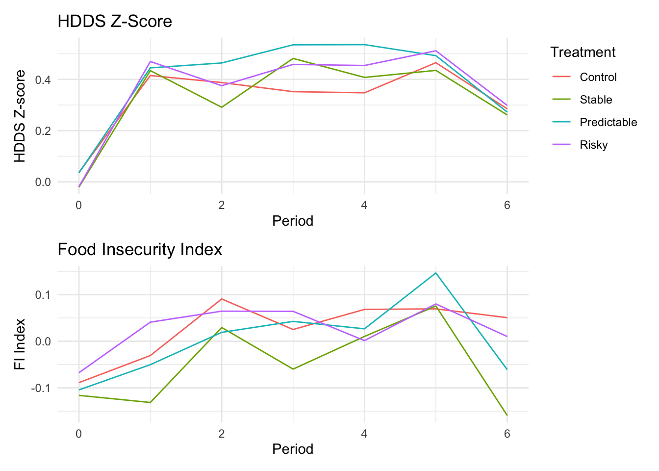
HDDS Z is a z-score of the FAO Household Dietary Diversity Score (HDDS). Higher score is better. The measure is a simple sum of the number of different food groups consumed in a given period.

Food Insecurity index is an Anderson index constructed from food insecurity questions. These questions are likert-scale questions about food insecurity experiences in the past period. A higher score indicates greater food insecurity.

1.6.1 Descriptive Graphs (mean)

Code
```{r}
#| label: fig-food-insecurity
#| fig-cap: "Food Insecurity Over Time"
#| warning: false
hdds_plot <- ggplot(df, aes(x = period, y = dd_hdds_z, color = treatment, group = treatment)) +
    geom_line(stat = "summary", fun = "mean") +
    labs(
        title = "HDDS Z-Score",
        x = "Period",
        y = "HDDS Z-score"
    ) +
    scale_color_discrete(
        name = "Treatment",
        labels = c("Control", "Stable", "Predictable", "Risky")
    ) +
    theme_minimal()

fi_plot <- ggplot(df, aes(x = period, y = fi_index_anderson, color = treatment, group = treatment)) +
    geom_line(stat = "summary", fun = "mean") +
    labs(
        title = "Food Insecurity Index",
        x = "Period",
        y = "FI Index"
    ) +
    scale_color_discrete(
        name = "Treatment",
        labels = c("Control", "Stable", "Predictable", "Risky")
    ) +
    theme_minimal()

(hdds_plot / fi_plot) + plot_layout(guides = "collect") & theme(legend.justification = c("right", "top"))
```
Figure 10: Food Insecurity Over Time

1.6.2 Period by Period Regression Coefficents

Code
```{r}
#| warning: false
#| message: false
hdds_reg_gp <- df %>%
    generate_coeff_df("dd_hdds_z") %>%
    effects_grapher("HDDS Z-Score")

fi_reg_gp <- df %>%
    generate_coeff_df("fi_index_anderson") %>%
    effects_grapher("FI Index")

(hdds_reg_gp / fi_reg_gp) + plot_layout(guides = "collect", axes = "collect") + plot_annotation(title = "Treatment effect on food insecurity")
```

1.6.3 Food Insecurity Regressions

Code
```{r}
#| label: tbl-food-insecurity-main
#| tbl-cap: ""
makeTable(c(
    models[["dd_hdds_z"]][1], models[["fi_index_anderson"]][1],
    models[["dd_hdds_z"]][3], models[["fi_index_anderson"]][3]
))
```
Table 46
HDDS Z-Score  FI Index HDDS Z-Score - Balanced Risky  FI Index - Balanced Risky
Stable 0.002 0.082** 0.002 0.084**
0.032 (−0.061, 0.065) 0.035 (0.014, 0.149) 0.032 (−0.061, 0.065) 0.035 (0.016, 0.152)
Predictable 0.053 0.049 0.052 0.048
0.033 (−0.012, 0.118) 0.036 (−0.021, 0.119) 0.033 (−0.014, 0.117) 0.036 (−0.023, 0.118)
Risky 0.033 0.030
0.027 (−0.021, 0.086) 0.029 (−0.027, 0.087)
Risky (Balanced) 0.023 0.007
0.036 (−0.047, 0.094) 0.041 (−0.072, 0.087)
Observations 14728 14728 9426 9426
Code
```{r}
#| label: tbl-food-insecurity-treatment-timing
#| tbl-cap: ""
makeTable(c(
    models[["dd_hdds_z"]][2], models[["fi_index_anderson"]][2]
))
```
Table 47
HDDS Z-Score - Anticipation Effect  FI Index - Anticipation Effect
Stable −0.002 0.048
0.035 (−0.072, 0.067) 0.039 (−0.029, 0.125)
Predictable Early 0.065 0.025
0.045 (−0.023, 0.154) 0.048 (−0.069, 0.118)
Predictable Late 0.068* 0.018
0.041 (−0.012, 0.149) 0.050 (−0.081, 0.117)
Risky Early 0.010 0.047
0.033 (−0.055, 0.075) 0.037 (−0.027, 0.120)
Risky Late 0.052 −0.010
0.033 (−0.012, 0.116) 0.038 (−0.084, 0.064)
Observations 10345 10345
Code
```{r}
#| label: tbl-food-insecurity-risky-splits
#| tbl-cap: ""
makeTable(c(
    models[["dd_hdds_z"]][4], models[["fi_index_anderson"]][4]
))
```
Table 48
HDDS Z-Score - Split Risky  FI Index - Split Risky
Stable 0.002 0.083**
0.032 (−0.061, 0.065) 0.035 (0.015, 0.151)
Predictable 0.054 0.045
0.033 (−0.011, 0.119) 0.036 (−0.025, 0.116)
Risky Medium 0.024 0.007
0.036 (−0.046, 0.094) 0.041 (−0.073, 0.086)
Risky High −0.021 −0.011
0.039 (−0.098, 0.056) 0.045 (−0.100, 0.078)
Risky Low 0.056 0.046
0.042 (−0.027, 0.139) 0.051 (−0.055, 0.146)
Observations 11492 11492
Code
```{r}
#| label: tbl-food-insecurity-income-interactions
#| tbl-cap: ""
makeTable(c(
    models[["dd_hdds_z"]][5], models[["fi_index_anderson"]][5],
    models[["dd_hdds_z"]][6], models[["fi_index_anderson"]][6],
    models[["dd_hdds_z"]][7], models[["fi_index_anderson"]][7]
))
```
Table 49
 HDDS Z-Score - Income  FI Index - Income  HDDS Z-Score - Income + Arm  FI Index - Income + Arm  HDDS Z-Score - Income X Arm  FI Index - Income X Arm
Stable 0.014 0.078** 0.033 0.048
0.033 (−0.051, 0.079) 0.036 (0.007, 0.149) 0.043 (−0.051, 0.117) 0.051 (−0.051, 0.147)
Predictable 0.065* 0.046 0.032 0.046
0.034 (−0.002, 0.132) 0.037 (−0.027, 0.118) 0.036 (−0.039, 0.103) 0.038 (−0.030, 0.121)
Risky 0.045 0.026 0.056* 0.028
0.028 (−0.011, 0.100) 0.030 (−0.033, 0.086) 0.029 (−0.001, 0.112) 0.031 (−0.033, 0.089)
Study Income −0.000 0.000 −0.000 0.000 −0.000** 0.000
0.000 (−0.000, 0.000) 0.000 (−0.000, 0.000) 0.000 (−0.000, 0.000) 0.000 (−0.000, 0.000) 0.000 (−0.001, −0.000) 0.000 (−0.000, 0.000)
Stable × Study Income −0.000 0.000
0.000 (−0.001, 0.001) 0.000 (−0.001, 0.001)
Predictable × Study Income 0.001** 0.000
0.000 (0.000, 0.001) 0.000 (−0.000, 0.001)
Observations 14728 14728 14728 14728 14728 14728
Note

For risky arms that did not complete dropoff, we impute a medium draw for the regressions below

Code
```{r}
#| label: tbl-food-insecurity-draw
#| tbl-cap: ""
makeTable(c(
    models[["dd_hdds_z"]][8], models[["fi_index_anderson"]][8],
    models[["dd_hdds_z"]][9], models[["fi_index_anderson"]][9]
))
```
Table 50
 HDDS Z-Score - Imputed Draw  FI Index - Imputed Draw  HDDS Z-Score - Imputed Draw with Lag  FI Index - Imputed Draw with Lag
High Draw 0.037 0.058 −0.709 −0.698
0.034 (−0.030, 0.104) 0.038 (−0.017, 0.134) 29211.557 (−57284.865, 57283.448) 34326.386 (−67315.087, 67313.690)
Medium Draw 0.021 0.060* −0.713 −0.697
0.030 (−0.038, 0.081) 0.033 (−0.004, 0.125) 29211.556 (−57284.869, 57283.442) 34326.385 (−67315.084, 67313.690)
Low Draw 0.045 0.071* −0.699 −0.686
0.034 (−0.022, 0.112) 0.038 (−0.004, 0.146) 29211.557 (−57284.856, 57283.458) 34326.386 (−67315.075, 67313.703)
High Draw previous period 0.740 0.745
29211.555 (−57283.412, 57284.893) 34326.383 (−67313.637, 67315.128)
Medium Draw previous period 0.737 0.746
29211.555 (−57283.417, 57284.890) 34326.385 (−67313.640, 67315.131)
Low Draw previous period 0.764 0.745
29211.554 (−57283.388, 57284.915) 34326.383 (−67313.638, 67315.127)
Observations 14728 14728 14728 14728
Note

Only treated participants that completed pickup are included in the regressions below.

Code
```{r}
#| label: tbl-food-insecurity-imputed-draw
#| tbl-cap: ""
makeTable(c(
    models[["dd_hdds_z"]][10], models[["fi_index_anderson"]][10],
    models[["dd_hdds_z"]][11], models[["fi_index_anderson"]][11]
))
```
Table 51
HDDS Z-Score - Realized Draw  FI Index - Realized Draw HDDS Z-Score - Realized Draw with Lag  FI Index - Realized Draw with Lag
High Draw 0.051 0.037 0.067* 0.035
0.036 (−0.020, 0.122) 0.040 (−0.042, 0.116) 0.038 (−0.006, 0.141) 0.042 (−0.047, 0.118)
Medium Draw −0.005 0.084** −0.003 0.078**
0.034 (−0.072, 0.062) 0.037 (0.010, 0.157) 0.035 (−0.071, 0.065) 0.039 (0.002, 0.154)
Low Draw 0.058 0.054 0.084** 0.038
0.036 (−0.012, 0.129) 0.040 (−0.024, 0.133) 0.039 (0.008, 0.159) 0.043 (−0.047, 0.122)
High Draw previous period −0.023 0.003
0.018 (−0.058, 0.012) 0.021 (−0.038, 0.043)
Observations 12335 12335 10755 10755
Note

Only participants who completed all surveys are included in the regressions below.

Code
```{r}
#| label: tbl-food-insecurity-balanced-panel
#| tbl-cap: ""
makeTable(c(
    models[["dd_hdds_z"]][12], models[["fi_index_anderson"]][12]
))
```
Table 52
HDDS Z-Score - Balanced Panel  FI Index - Balanced Panel
Stable 0.010 0.058
0.040 (−0.068, 0.089) 0.044 (−0.028, 0.143)
Predictable 0.048 0.046
0.041 (−0.033, 0.129) 0.046 (−0.044, 0.135)
Risky 0.055 0.000
0.034 (−0.013, 0.122) 0.038 (−0.074, 0.074)
Observations 10493 10493
Note

The regressions below include baseline (period 0) data.

Code
```{r}
#| label: tbl-food-insecurity-baseline-included
#| tbl-cap: ""
makeTable(c(
    models[["dd_hdds_z"]][16], models[["fi_index_anderson"]][16]
))
```
Table 53
 HDDS Z-Score - Baseline Included  FI Index - Baseline Included
Stable 0.007 0.070**
0.028 (−0.049, 0.063) 0.030 (0.011, 0.130)
Predictable 0.049* 0.043
0.029 (−0.008, 0.107) 0.032 (−0.019, 0.104)
Risky 0.031 0.024
0.024 (−0.016, 0.078) 0.025 (−0.026, 0.074)
Observations 17000 17000
Note

The regressions below exclude endline (period 6) data.

Code
```{r}
#| label: tbl-food-insecurity-excluding-endline
#| tbl-cap: ""
makeTable(c(
    models[["dd_hdds_z"]][17], models[["fi_index_anderson"]][17]
))
```
Table 54
HDDS Z-Score - Excluding Endline  FI Index - Excluding Endline
Stable −0.002 0.048
0.035 (−0.072, 0.067) 0.039 (−0.029, 0.125)
Predictable 0.067* 0.022
0.036 (−0.003, 0.136) 0.040 (−0.057, 0.100)
Risky 0.031 0.019
0.030 (−0.028, 0.089) 0.033 (−0.047, 0.084)
Observations 10345 10345

2 Visual Results

Code
```{r}
#| output: false
#| warning: false
#| message: false
model_to_coef_treatment <- function(var) {
    varName <- ifelse(var == "phq2_z" | var == "gad2_z", var, paste0(var, "_z"))
    coeff_df <- z_models[[varName]][[1]] %>%
        tidy(, conf.int = T) %>%
        filter(str_detect(term, "treatment")) %>%
        mutate(
            treatment = case_when(
                term == "treatment::1" ~ "Stable",
                term == "treatment::2" ~ "Predictable",
                term == "treatment::3" ~ "Risky",
            ),
            variable = variableLabels[[var]],
            # Compute average estimate for sorting
            avg_estimate = mean(estimate)
        ) %>%
        select(!c(term))
    coeff_df
}

model_to_coef_treatment_timing <- function(var) {
    varName <- ifelse(var == "phq2_z" | var == "gad2_z", var, paste0(var, "_z"))
    coeff_df <- z_models[[varName]][[2]] %>%
        tidy(, conf.int = T) %>%
        filter(str_detect(term, "treatment_timing")) %>%
        mutate(
            treatment = case_when(
                term == "treatment_timing::1" ~ "Stable",
                term == "treatment_timing::2" ~ "Predictable Early",
                term == "treatment_timing::3" ~ "Predictable Late",
                term == "treatment_timing::4" ~ "Risky Early",
                term == "treatment_timing::5" ~ "Risky Late"
            ),
            variable = variableLabels[[var]],
            # Compute average estimate for sorting
            avg_estimate = mean(estimate)
        ) %>%
        select(!c(term))
    coeff_df
}


model_to_coef_treatment_split <- function(var) {
    varName <- ifelse(var == "phq2_z" | var == "gad2_z", var, paste0(var, "_z"))
    coeff_df <- z_models[[varName]][[4]] %>%
        tidy(, conf.int = T) %>%
        filter(str_detect(term, "treatment_split")) %>%
        mutate(
            treatment = case_when(
                term == "treatment_split::1" ~ "Stable",
                term == "treatment_split::2" ~ "Predictable",
                term == "treatment_split::3" ~ "Risky Medium",
                term == "treatment_split::4" ~ "Risky High",
                term == "treatment_split::5" ~ "Risky Low"
            ),
            variable = variableLabels[[var]],
            # Compute average estimate for sorting
            avg_estimate = mean(estimate)
        ) %>%
        select(!c(term))
    coeff_df
}

model_to_coef_draw <- function(var) {
    varName <- ifelse(var == "phq2_z" | var == "gad2_z", var, paste0(var, "_z"))
    coeff_df <- z_models[[varName]][[10]] %>%
        tidy(, conf.int = T) %>%
        filter(str_detect(term, "draw_realized")) %>%
        mutate(
            draw = case_when(
                term == "draw_realized::H" ~ "High",
                term == "draw_realized::M" ~ "Medium",
                term == "draw_realized::L" ~ "Low",
                .default = term
            ),
            variable = variableLabels[[var]],
            # Compute average estimate for sorting
            avg_estimate = mean(estimate)
        ) %>%
        select(!c(term))
    coeff_df
}
```
Code
```{r, fig.height=9, fig.width = 7}
treatment_results <- map(variables, model_to_coef_treatment) %>%
    bind_rows() %>%
    mutate(variable = fct_reorder(variable, avg_estimate)) %>%
    # sort by avg_estimate
    arrange(avg_estimate)

ggplot(treatment_results, aes(y = treatment, x = estimate, group = treatment, color = treatment)) +
    geom_pointrange(aes(xmin = conf.low, xmax = conf.high)) +
    facet_grid(variable ~ ., scales = "free_y", space = "free_y", switch = "y") +
    geom_vline(xintercept = 0, color = "grey") +
    ylab(NULL) +
    xlab("Estimated Effect (SD)") +
    theme(
        axis.text.y = element_blank(),
        axis.ticks.y = element_blank(),
        strip.placement = "outside",
        strip.background = element_blank(),
        strip.text.y.left = element_text(angle = 0, hjust = 0)
    )
```

Code
```{r, fig.height=12, fig.width = 7}
treatment_results_timing <- map(variables, model_to_coef_treatment_timing) %>%
    bind_rows() %>%
    mutate(
        variable = fct_reorder(variable, avg_estimate),
        treatment = fct_reorder(
            treatment,
            case_when(
                treatment == "Stable" ~ 1,
                treatment == "Predictable Late" ~ 2,
                treatment == "Predictable Early" ~ 3,
                treatment == "Risky Late" ~ 4,
                treatment == "Risky Early" ~ 5,
                TRUE ~ NA_real_
            )
        )
    ) %>%
    # sort by avg_estimate
    arrange(avg_estimate)

ggplot(treatment_results_timing, aes(y = treatment, x = estimate, group = treatment, color = treatment)) +
    geom_pointrange(aes(xmin = conf.low, xmax = conf.high)) +
    facet_grid(variable ~ ., scales = "free_y", space = "free_y", switch = "y") +
    geom_vline(xintercept = 0, color = "grey") +
    ylab(NULL) +
    xlab("Estimated Effect (SD)") +
    theme(
        axis.text.y = element_blank(),
        axis.ticks.y = element_blank(),
        strip.placement = "outside",
        strip.background = element_blank(),
        strip.text.y.left = element_text(angle = 0, hjust = 0)
    )
```

Note

The coefficents below only include people who completed all 6 surveys

Code
```{r, fig.height=9, fig.width = 7}
model_to_coef_balanced <- function(var) {
    varName <- ifelse(var == "phq2_z" | var == "gad2_z", var, paste0(var, "_z"))
    coeff_df <- z_models[[varName]][[12]] %>%
        tidy(, conf.int = T) %>%
        filter(str_detect(term, "treatment")) %>%
        mutate(
            treatment = case_when(
                term == "treatment::1" ~ "Stable",
                term == "treatment::2" ~ "Predictable",
                term == "treatment::3" ~ "Risky",
            ),
            variable = variableLabels[[var]],
            # Compute average estimate for sorting
            avg_estimate = mean(estimate)
        ) %>%
        select(!c(term))
    coeff_df
}

treatment_balanced <- map(variables, model_to_coef_balanced) %>%
    bind_rows() %>%
    mutate(variable = fct_reorder(variable, avg_estimate)) %>%
    # sort by avg_estimate
    arrange(avg_estimate)

ggplot(treatment_balanced, aes(y = treatment, x = estimate, group = treatment, color = treatment)) +
    geom_pointrange(aes(xmin = conf.low, xmax = conf.high)) +
    facet_grid(variable ~ ., scales = "free_y", space = "free_y", switch = "y") +
    geom_vline(xintercept = 0, color = "grey") +
    ylab(NULL) +
    xlab("Estimated Effect (SD)") +
    theme(
        axis.text.y = element_blank(),
        axis.ticks.y = element_blank(),
        strip.placement = "outside",
        strip.background = element_blank(),
        strip.text.y.left = element_text(angle = 0, hjust = 0)
    )
```

Code
```{r, fig.height=12, fig.width = 7}
treatment_results_split <- map(variables, model_to_coef_treatment_split) %>%
    bind_rows() %>%
    mutate(
        variable = fct_reorder(variable, avg_estimate),
        # Reorder treatment so 1 - Stable 2 - Predictable 3 - Risky low 4 - Risky Medium 5 - Risky High
        treatment = fct_reorder(
            treatment,
            case_when(
                treatment == "Stable" ~ 1,
                treatment == "Predictable" ~ 2,
                treatment == "Risky Low" ~ 3,
                treatment == "Risky Medium" ~ 4,
                treatment == "Risky High" ~ 5,
                TRUE ~ NA_real_
            )
        )
    ) %>%
    # sort by avg_estimate
    arrange(avg_estimate)

ggplot(treatment_results_split, aes(y = treatment, x = estimate, group = treatment, color = treatment)) +
    geom_pointrange(aes(xmin = conf.low, xmax = conf.high)) +
    facet_grid(variable ~ ., scales = "free_y", space = "free_y", switch = "y") +
    geom_vline(xintercept = 0, color = "grey") +
    ylab(NULL) +
    xlab("Estimated Effect (SD)") +
    theme(
        axis.text.y = element_blank(),
        axis.ticks.y = element_blank(),
        strip.placement = "outside",
        strip.background = element_blank(),
        strip.text.y.left = element_text(angle = 0, hjust = 0)
    )
```

Code
```{r, fig.height=9, fig.width = 7}
treatment_results_draw <- map(variables, model_to_coef_draw) %>%
    bind_rows() %>%
    mutate(
        variable = fct_reorder(variable, avg_estimate),
        draw = fct_reorder(
            draw,
            case_when(
                draw == "Low" ~ 1,
                draw == "Medium" ~ 2,
                draw == "High" ~ 3,
                TRUE ~ NA_real_
            )
        )
    ) %>%
    # sort by avg_estimate
    arrange(avg_estimate)

ggplot(treatment_results_draw, aes(y = draw, x = estimate, group = draw, color = draw)) +
    geom_pointrange(aes(xmin = conf.low, xmax = conf.high)) +
    facet_grid(variable ~ ., scales = "free_y", space = "free_y", switch = "y") +
    geom_vline(xintercept = 0, color = "grey") +
    ylab(NULL) +
    xlab("Estimated Effect (SD)") +
    theme(
        axis.text.y = element_blank(),
        axis.ticks.y = element_blank(),
        strip.placement = "outside",
        strip.background = element_blank(),
        strip.text.y.left = element_text(angle = 0, hjust = 0)
    )
```

Note

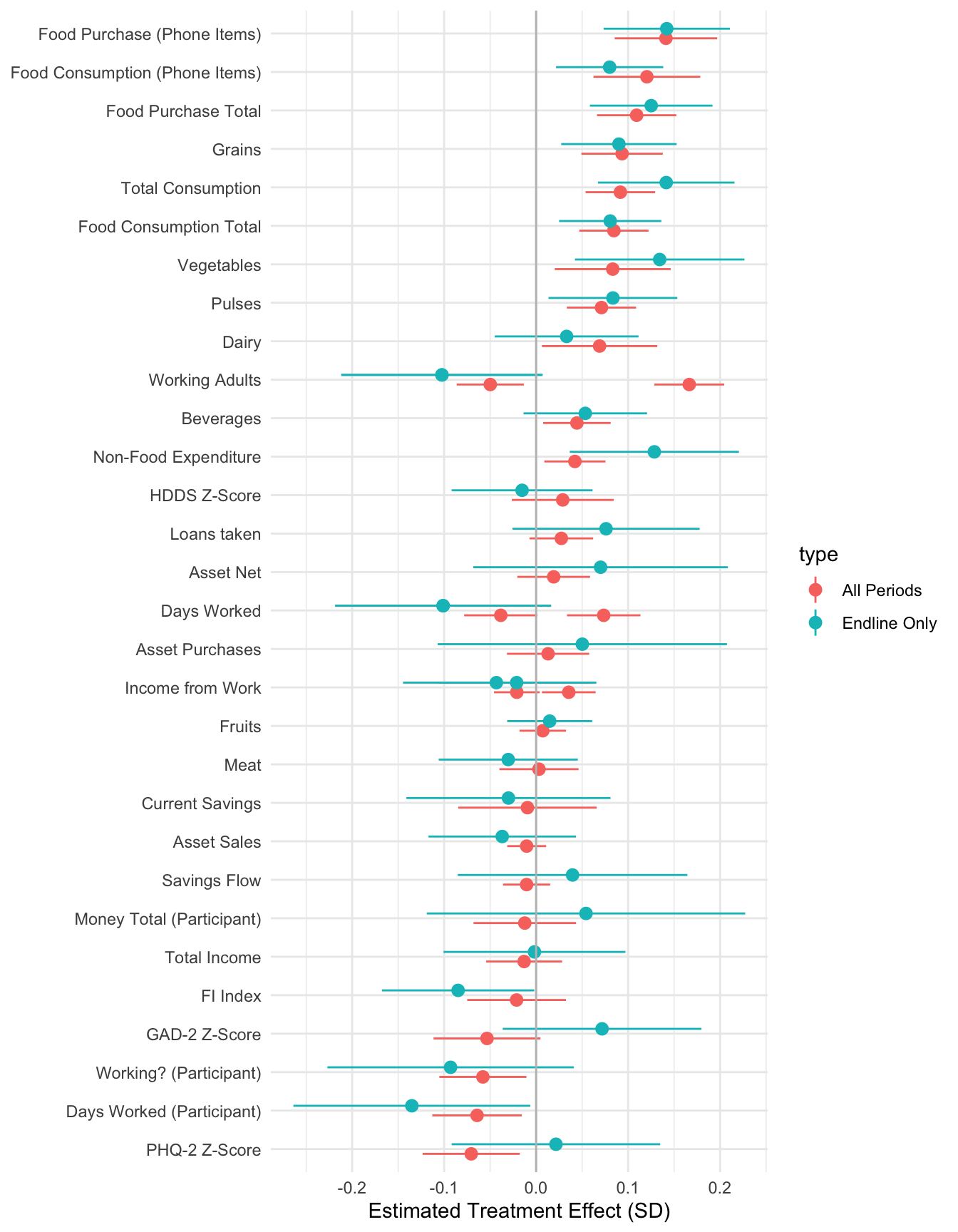
The following results only include data from the endline and thus do not have period fixed effects. They are othwerwise identical to the main treatment results.

Code
```{r, fig.height=9, fig.width = 7}
model_to_coef_endline <- function(var) {
    varName <- ifelse(var == "phq2_z" | var == "gad2_z", var, paste0(var, "_z"))
    coeff_df <- z_models[[varName]][[13]] %>%
        tidy(conf.int = T) %>%
        filter(str_detect(term, "treatment")) %>%
        mutate(
            treatment = case_when(
                term == "treatment::1" ~ "Stable",
                term == "treatment::2" ~ "Predictable",
                term == "treatment::3" ~ "Risky",
            ),
            variable = variableLabels[[var]],
            # Compute average estimate for sorting
            avg_estimate = mean(estimate)
        ) %>%
        select(!c(term))
    coeff_df
}

treatment_results_endline <- map(variables, model_to_coef_endline) %>%
    bind_rows() %>%
    mutate(
        variable = fct_reorder(variable, avg_estimate),
        # Reorder treatment so 1 - Stable 2 - Predictable 3 - Risky low 4 - Risky Medium 5 - Risky High
        treatment = fct_reorder(
            treatment,
            case_when(
                treatment == "Stable" ~ 1,
                treatment == "Preidctable" ~ 2,
                treatment == "Risky" ~ 3,
                .default = 4
            )
        )
    ) %>%
    # sort by avg_estimate
    arrange(avg_estimate)

ggplot(treatment_results_endline, aes(y = treatment, x = estimate, group = treatment, color = treatment)) +
    geom_pointrange(aes(xmin = conf.low, xmax = conf.high)) +
    facet_grid(variable ~ ., scales = "free_y", space = "free_y", switch = "y") +
    geom_vline(xintercept = 0, color = "grey") +
    ylab(NULL) +
    xlab("Estimated Effect (SD)") +
    theme(
        axis.text.y = element_blank(),
        axis.ticks.y = element_blank(),
        strip.placement = "outside",
        strip.background = element_blank(),
        strip.text.y.left = element_text(angle = 0, hjust = 0)
    )
```

Code
```{r, fig.height=9, fig.width = 7}
model_to_coef_tvc <- function(var) {
    varName <- ifelse(var == "phq2_z" | var == "gad2_z", var, paste0(var, "_z"))
    coeff_df <- z_models[[varName]][[14]] %>%
        tidy(, conf.int = T) %>%
        filter(str_detect(term, "treated")) %>%
        mutate(
            variable = variableLabels[var],
            type = "All Periods"
        ) %>%
        select(!c(term))
    endline_df <- z_models[[varName]][[15]] %>%
        tidy(, conf.int = T) %>%
        filter(str_detect(term, "treated")) %>%
        mutate(
            variable = variableLabels[var],
            type = "Endline Only"
        ) %>%
        select(!c(term))
    # Append endline_df and coeff_df
    coeff_df <- bind_rows(coeff_df, endline_df) %>%
        mutate(
            # Set the sort to be based type == All Periods coefficients
            sort_estimate = max(ifelse(type == "All Periods", estimate, NA_real_), na.rm = T)
        )

    coeff_df
}


control_coefs <- map(variables, model_to_coef_tvc) %>%
    bind_rows() %>%
    mutate(variable = fct_reorder(variable, sort_estimate))

ggplot(control_coefs, aes(x = variable, y = estimate, group = type, color = type)) +
    geom_pointrange(aes(ymin = conf.low, ymax = conf.high), position = position_dodge(width = 0.5)) +
    geom_hline(yintercept = 0, color = "grey") +
    coord_flip() +
    xlab(NULL) +
    ylab("Estimated Treatment Effect (SD)")
```

3 Appendix

3.1 Log Food Consumption and Expenditure

Code
```{r}
#| label: tbl-log-consumption-expenditure
#| tbl-cap: "Treatment Effects on Log Food Consumption and Non-Food Expenditure (Excluding Endline)"
#| warning: false
#| message: false

# Create log versions of food consumption and non-food expenditure
df <- df %>%
    mutate(
        log_food_consumption_total_99 = log(food_consumption_total_99 + 1),
        log_expenditure_total_nonfood_99 = log(expenditure_total_nonfood_99 + 1),
        log_food_consumption_total_99_bl = log(food_consumption_total_99_bl + 1),
        log_expenditure_total_nonfood_99_bl = log(expenditure_total_nonfood_99_bl + 1)
    )

# Run regressions for log food consumption
log_food_consumption_reg <- feols(
    log_food_consumption_total_99 ~ log_food_consumption_total_99_bl + hh_size + census_wealth_index + i(treatment) | district_id + period + wave + enum_id + day_of_week + cohort,
    cluster = "hh_id",
    data = df %>% filter(period > 0 & period < 6)
)

# Run regressions for log non-food expenditure
log_nonfood_expenditure_reg <- feols(
    log_expenditure_total_nonfood_99 ~ log_expenditure_total_nonfood_99_bl + hh_size + census_wealth_index + i(treatment) | district_id + period + wave + enum_id + day_of_week + cohort,
    cluster = "hh_id",
    data = df %>% filter(period > 0 & period < 6)
)

modelsummary(
    list(
        "Log Food Consumption" = log_food_consumption_reg,
        "Log Non-Food Expenditure" = log_nonfood_expenditure_reg
    ),
    title = "Treatment Effects (Excluding Endline)",
    escape = FALSE,
    output = "kableExtra",
    estimate = "{estimate}{stars}",
    statistic = "{std.error} ({conf.low}, {conf.high})",
    coef_omit = NULL,
    coef_omit_sources = FALSE,
    stars = c(`***` = 0.01, `**` = 0.05, `*` = 0.1),
    gof_map = tribble(
        ~raw, ~clean, ~fmt,
        "nobs", "Observations", 0,
        "FE", "Fixed Effects", 1,
    ),
    coef_rename = c(
        "log_food_consumption_total_99_bl" = "Baseline (log)",
        "log_expenditure_total_nonfood_99_bl" = "Baseline (log)",
        "hh_size" = "Household Size",
        "census_wealth_index" = "Wealth Index",
        "treatment::1" = "Stable",
        "treatment::2" = "Predictable",
        "treatment::3" = "Risky"
    )
) %>%
    kable_classic(full_width = F, html_font = "Cambria", fixed_thead = T)
```
Table 55: Treatment Effects on Log Food Consumption and Non-Food Expenditure (Excluding Endline)
Treatment Effects (Excluding Endline)
Log Food Consumption Log Non-Food Expenditure
Baseline (log) 0.205*** 0.080***
0.013 (0.178, 0.231) 0.011 (0.058, 0.102)
Household Size 0.020*** 0.022***
0.003 (0.015, 0.026) 0.006 (0.011, 0.033)
Wealth Index 0.038*** 0.036
0.012 (0.013, 0.062) 0.026 (−0.014, 0.087)
Stable 0.047* 0.087*
0.026 (−0.003, 0.098) 0.051 (−0.013, 0.186)
Predictable 0.087*** 0.069
0.025 (0.038, 0.137) 0.053 (−0.035, 0.173)
Risky 0.062*** 0.032
0.021 (0.020, 0.103) 0.043 (−0.052, 0.116)
Observations 10345 10309

3.2 Instrumented Income

Note

See Income and Days Worked Section for descriptives and details of the income variable

3.2.1 Income Effects on Consumption

Code
```{r}
#| label: model-consumption-instrumented-income
#| warning: false
#| message: false

## Copied from main regressions; adjuts if chagned
# Define common fixed effects specification

income <- feols(total_consumption_99 ~ total_consumption_99_bl + hh_size + census_wealth_index + total_income_99 * i(treatment, ref = 0) | community_id + period,
    cluster = "community_id",
    data = df,
    collin.tol = 1e-5
)

study_income <- feols(total_consumption_99 ~ total_consumption_99_bl + hh_size + census_wealth_index + study_income * i(treatment, ref = 0) | community_id + period,
    cluster = "community_id",
    data = df,
    collin.tol = 1e-5
)

work_income <- feols(total_consumption_99 ~ total_consumption_99_bl + hh_size + census_wealth_index + money_work_corrected_99 * i(treatment, ref = 0) | community_id + period,
    cluster = "community_id",
    data = df,
    collin.tol = 1e-5
)

work_income_p <- feols(total_consumption_99 ~ total_consumption_99_bl + hh_size + census_wealth_index + money_earn_p_corrected * i(treatment, ref = 0) | community_id + period,
    cluster = "community_id",
    data = df,
    collin.tol = 1e-5
)

# Instrument Participant Income
instrumented_work_income_p <- feols(total_consumption_99 ~ total_consumption_99_bl + hh_size + census_wealth_index + i(treatment, ref = 0) | community_id + period | money_earn_p_corrected:i(treatment, ref = 0) + money_earn_p_corrected ~ study_income:i(treatment, ref = 0) + study_income,
    cluster = "community_id",
    data = df,
    collin.tol = 1e-5
)
# Instrument work Income
instrumented_work_income <- feols(total_consumption_99 ~ total_consumption_99_bl + hh_size + census_wealth_index + i(treatment, ref = 0) | community_id + period | money_work_corrected_99:i(treatment, ref = 0) + money_work_corrected_99 ~ study_income:i(treatment, ref = 0) + study_income,
    cluster = "community_id",
    data = df,
    collin.tol = 1e-5
)
# Instrument Total Income
instrumented_income <- feols(total_consumption_99 ~ total_consumption_99_bl + hh_size + census_wealth_index + i(treatment, ref = 0) | community_id + period | total_income_99:i(treatment, ref = 0) + total_income_99 ~ study_income:i(treatment, ref = 0) + study_income,
    cluster = "community_id",
    data = df,
    collin.tol = 1e-5
)


income_hh_fe <- feols(total_consumption_99 ~ total_consumption_99_bl + hh_size + census_wealth_index + total_income_99 * i(treatment, ref = 0) | period + hh_id,
    cluster = "community_id",
    data = df,
    collin.tol = 1e-5
)

instrumented_income_hh_fe <- feols(total_consumption_99 ~ 1 | hh_id + period | total_income_99:i(treatment, ref = 0) + total_income_99 ~ study_income:i(treatment, ref = 0) + study_income,
    cluster = "community_id",
    data = df,
    collin.tol = 1e-5
)

modelsummary(
    list(
        "Study Income" = study_income,
        "Total Income" = income,
        "Total Income (instrumented)" = instrumented_income,
        "Work Income" = work_income,
        "Work Income (instrumented)" = instrumented_work_income,
        "Participant Work Income" = work_income_p,
        "Participant Work Income (instrumented)" = instrumented_work_income_p,
        "Total Income + HH FE" = income_hh_fe,
        "Total Income + HH FE (instrumented)" = instrumented_income_hh_fe
    ),
    title = "Treatment Effects on Consumption",
    escape = FALSE,
    output = "kableExtra",
    estimate = "{estimate}{stars}",
    statistic = "{std.error} ({conf.low}, {conf.high})",
    coef_omit = NULL,
    coef_omit_sources = FALSE,
    stars = c(`***` = 0.01, `**` = 0.05, `*` = 0.1),
    gof_map = tribble(
        ~raw, ~clean, ~fmt,
        "nobs", "Observations", 0,
        "FE", "Community FE", 1,
    ),
    # rename all the fit_ variables from the instrumentation so that the table is cleaner
    coef_rename = c(
        "total_consumption_99_bl" = "Baseline Consumption",
        "hh_size" = "Household Size",
        "census_wealth_index" = "Wealth Index",
        "money_work_corrected_99" = "Income",
        "money_earn_p_corrected" = "Income",
        "total_income_99" = "Income",
        "fit_money_work_corrected_99" = "Income",
        "fit_money_earn_p_corrected" = "Income",
        "fit_total_income_99" = "Income",
        "treatment::1" = "Stable",
        "treatment::2" = "Predictable",
        "treatment::3" = "Risky",
        # rename all interactions
        "money_work_corrected_99:treatment::1" = "Income x Stable",
        "money_work_corrected_99:treatment::2" = "Income x Predictable",
        "money_work_corrected_99:treatment::3" = "Income x Risky",
        "fit_money_work_corrected_99:treatment::1" = "Income x Stable",
        "fit_money_work_corrected_99:treatment::2" = "Income x Predictable",
        "fit_money_work_corrected_99:treatment::3" = "Income x Risky",
        "money_earn_p_corrected:treatment::1" = "Income x Stable",
        "money_earn_p_corrected:treatment::2" = "Income x Predictable",
        "money_earn_p_corrected:treatment::3" = "Income x Risky",
        "fit_money_earn_p_corrected:treatment::1" = "Income x Stable",
        "fit_money_earn_p_corrected:treatment::2" = "Income x Predictable",
        "fit_money_earn_p_corrected:treatment::3" = "Income x Risky",
        "total_income_99:treatment::1" = "Income x Stable",
        "total_income_99:treatment::2" = "Income x Predictable",
        "total_income_99:treatment::3" = "Income x Risky",
        "fit_total_income_99:treatment::1" = "Income x Stable",
        "fit_total_income_99:treatment::2" = "Income x Predictable",
        "fit_total_income_99:treatment::3" = "Income x Risky"
    )
) %>%
    kable_classic(full_width = F, html_font = "Cambria", fixed_thead = T)
```
Treatment Effects on Consumption
 Study Income  Total Income  Total Income (instrumented)  Work Income  Work Income (instrumented)  Participant Work Income  Participant Work Income (instrumented)  Total Income + HH FE  Total Income + HH FE (instrumented)
Baseline Consumption 0.252*** 0.246*** 0.360 0.251*** 0.239*** 0.251*** 0.263***
0.010 (0.231, 0.272) 0.010 (0.225, 0.266) 0.756 (−1.138, 1.858) 0.010 (0.230, 0.272) 0.026 (0.186, 0.291) 0.010 (0.230, 0.272) 0.019 (0.225, 0.301)
Household Size 11.262*** 10.724*** 20.215 10.942*** 6.584 11.236*** 12.354***
1.835 (7.628, 14.896) 1.813 (7.133, 14.314) 64.105 (−106.764, 147.194) 1.839 (7.300, 14.584) 8.041 (−9.344, 22.513) 1.819 (7.633, 14.840) 2.303 (7.792, 16.916)
Wealth Index 16.100* 12.349 88.734 14.557 −9.127 15.337* 21.823**
9.174 (−2.073, 34.273) 9.058 (−5.594, 30.291) 512.725 (−926.875, 1104.344) 9.155 (−3.578, 32.692) 49.111 (−106.406, 88.153) 9.184 (−2.854, 33.529) 10.762 (0.506, 43.140)
study_income −0.062
0.082 (−0.224, 0.100)
Stable 36.983** 54.864*** 72.800 55.795*** 94.260 53.434*** 58.522
15.296 (6.685, 67.280) 17.122 (20.948, 88.780) 330.764 (−582.379, 727.979) 16.858 (22.403, 89.188) 75.186 (−54.669, 243.188) 16.097 (21.549, 85.320) 51.606 (−43.700, 160.744)
Predictable 38.928** 39.546** 1321.731 51.003*** −141.119 51.202*** 69.399
15.319 (8.585, 69.272) 15.860 (8.130, 70.962) 8336.123 (−15190.525, 17833.986) 15.257 (20.783, 81.224) 475.415 (−1082.824, 800.587) 14.601 (22.280, 80.124) 63.233 (−55.853, 194.651)
Risky 47.956*** 44.559*** 45.724*** 47.596***
12.500 (23.195, 72.716) 11.932 (20.923, 68.195) 12.419 (21.125, 70.324) 12.128 (23.574, 71.618)
study_income:treatment::1 0.242
0.213 (−0.180, 0.664)
study_income:treatment::2 0.186
0.132 (−0.075, 0.447)
Income 0.124*** −1.136 0.216*** 1.428 0.530** −2.098 0.104*** −0.325
0.028 (0.069, 0.179) 8.218 (−17.415, 15.142) 0.068 (0.081, 0.351) 3.190 (−4.890, 7.746) 0.267 (0.001, 1.058) 3.774 (−9.573, 5.376) 0.027 (0.051, 0.158) 0.640 (−1.593, 0.943)
Income x Stable −0.022 −0.101 −0.112 −0.952 −0.370 −0.151 −0.026 −0.229
0.034 (−0.090, 0.046) 1.617 (−3.303, 3.101) 0.093 (−0.296, 0.072) 1.546 (−4.014, 2.110) 0.268 (−0.901, 0.161) 4.549 (−9.163, 8.860) 0.040 (−0.105, 0.053) 0.336 (−0.895, 0.436)
Income x Predictable 0.023 −5.271 −0.048 4.629 −0.416 −0.535 0.029 −1.260
0.034 (−0.045, 0.090) 34.453 (−73.515, 62.973) 0.092 (−0.230, 0.134) 11.643 (−18.432, 27.691) 0.265 (−0.942, 0.109) 4.922 (−10.285, 9.214) 0.032 (−0.035, 0.093) 2.709 (−6.627, 4.107)
Income x Risky −0.002 0.164 −0.022 1.220** −0.428 4.240*** 0.007 0.095
0.027 (−0.055, 0.052) 0.341 (−0.512, 0.840) 0.074 (−0.168, 0.123) 0.509 (0.211, 2.228) 0.274 (−0.971, 0.115) 1.389 (1.489, 6.992) 0.030 (−0.052, 0.066) 0.577 (−1.048, 1.239)
Observations 17000 17000 17000 17000 17000 17000 17000 16998 16998

3.2.2 Income Effects on Non-Food Expenditure

Code
```{r}
#| label: model-non-food-expenditure-instrumented-income
#| warning: false
#| message: false

## Copied from main regressions; adjuts if chagned
# Define common fixed effects specification
income <- feols(expenditure_total_nonfood_99 ~ expenditure_total_nonfood_99_bl + hh_size + census_wealth_index + total_income_99 * i(treatment, ref = 0) | community_id + period,
    cluster = "community_id",
    data = df,
    collin.tol = 1e-5
)

study_income <- feols(expenditure_total_nonfood_99 ~ expenditure_total_nonfood_99_bl + hh_size + census_wealth_index + study_income * i(treatment, ref = 0) | community_id + period,
    cluster = "community_id",
    data = df,
    collin.tol = 1e-5
)

work_income <- feols(expenditure_total_nonfood_99 ~ expenditure_total_nonfood_99_bl + hh_size + census_wealth_index + money_work_corrected_99 * i(treatment, ref = 0) | community_id + period,
    cluster = "community_id",
    data = df,
    collin.tol = 1e-5
)

work_income_p <- feols(expenditure_total_nonfood_99 ~ expenditure_total_nonfood_99_bl + hh_size + census_wealth_index + money_earn_p_corrected * i(treatment, ref = 0) | community_id + period,
    cluster = "community_id",
    data = df,
    collin.tol = 1e-5
)

# Instrument Participant Income
instrumented_work_income_p <- feols(expenditure_total_nonfood_99 ~ expenditure_total_nonfood_99_bl + hh_size + census_wealth_index + i(treatment, ref = 0) | community_id + period | money_earn_p_corrected:i(treatment, ref = 0) + money_earn_p_corrected ~ study_income:i(treatment, ref = 0) + study_income,
    cluster = "community_id",
    data = df,
    collin.tol = 1e-5
)
# Instrument work Income
instrumented_work_income <- feols(expenditure_total_nonfood_99 ~ expenditure_total_nonfood_99_bl + hh_size + census_wealth_index + i(treatment, ref = 0) | community_id + period | money_work_corrected_99:i(treatment, ref = 0) + money_work_corrected_99 ~ study_income:i(treatment, ref = 0) + study_income,
    cluster = "community_id",
    data = df,
    collin.tol = 1e-5
)
# Instrument Total Income
instrumented_income <- feols(expenditure_total_nonfood_99 ~ expenditure_total_nonfood_99_bl + hh_size + census_wealth_index + i(treatment, ref = 0) | community_id + period | total_income_99:i(treatment, ref = 0) + total_income_99 ~ study_income:i(treatment, ref = 0) + study_income,
    cluster = "community_id",
    data = df,
    collin.tol = 1e-5
)


income_hh_fe <- feols(expenditure_total_nonfood_99 ~ expenditure_total_nonfood_99_bl + hh_size + census_wealth_index + total_income_99 * i(treatment, ref = 0) | period + hh_id,
    cluster = "community_id",
    data = df,
    collin.tol = 1e-5
)

instrumented_income_hh_fe <- feols(expenditure_total_nonfood_99 ~ 1 | hh_id + period | total_income_99:i(treatment, ref = 0) + total_income_99 ~ study_income:i(treatment, ref = 0) + study_income,
    cluster = "community_id",
    data = df,
    collin.tol = 1e-5
)

modelsummary(
    list(
        "Study Income" = study_income,
        "Total Income" = income,
        "Total Income (instrumented)" = instrumented_income,
        "Work Income" = work_income,
        "Work Income (instrumented)" = instrumented_work_income,
        "Participant Work Income" = work_income_p,
        "Participant Work Income (instrumented)" = instrumented_work_income_p,
        "Total Income + HH FE" = income_hh_fe,
        "Total Income + HH FE (instrumented)" = instrumented_income_hh_fe
    ),
    title = "Treatment Effects on Non-Food Expenditure",
    escape = FALSE,
    output = "kableExtra",
    estimate = "{estimate}{stars}",
    statistic = "{std.error} ({conf.low}, {conf.high})",
    coef_omit = NULL,
    coef_omit_sources = FALSE,
    stars = c(`***` = 0.01, `**` = 0.05, `*` = 0.1),
    gof_map = tribble(
        ~raw, ~clean, ~fmt,
        "nobs", "Observations", 0,
        "FE", "Community FE", 1,
    ),
    # rename all the fit_ variables from the instrumentation so that the table is cleaner
    coef_rename = c(
        "total_consumption_99_bl" = "Baseline Consumption",
        "hh_size" = "Household Size",
        "census_wealth_index" = "Wealth Index",
        "money_work_corrected_99" = "Income",
        "money_earn_p_corrected" = "Income",
        "total_income_99" = "Income",
        "fit_money_work_corrected_99" = "Income",
        "fit_money_earn_p_corrected" = "Income",
        "fit_total_income_99" = "Income",
        "treatment::1" = "Stable",
        "treatment::2" = "Predictable",
        "treatment::3" = "Risky",
        # rename all interactions
        "money_work_corrected_99:treatment::1" = "Income x Stable",
        "money_work_corrected_99:treatment::2" = "Income x Predictable",
        "money_work_corrected_99:treatment::3" = "Income x Risky",
        "fit_money_work_corrected_99:treatment::1" = "Income x Stable",
        "fit_money_work_corrected_99:treatment::2" = "Income x Predictable",
        "fit_money_work_corrected_99:treatment::3" = "Income x Risky",
        "money_earn_p_corrected:treatment::1" = "Income x Stable",
        "money_earn_p_corrected:treatment::2" = "Income x Predictable",
        "money_earn_p_corrected:treatment::3" = "Income x Risky",
        "fit_money_earn_p_corrected:treatment::1" = "Income x Stable",
        "fit_money_earn_p_corrected:treatment::2" = "Income x Predictable",
        "fit_money_earn_p_corrected:treatment::3" = "Income x Risky",
        "total_income_99:treatment::1" = "Income x Stable",
        "total_income_99:treatment::2" = "Income x Predictable",
        "total_income_99:treatment::3" = "Income x Risky",
        "fit_total_income_99:treatment::1" = "Income x Stable",
        "fit_total_income_99:treatment::2" = "Income x Predictable",
        "fit_total_income_99:treatment::3" = "Income x Risky"
    )
) %>%
    kable_classic(full_width = F, html_font = "Cambria", fixed_thead = T)
```
Treatment Effects on Non-Food Expenditure
 Study Income  Total Income  Total Income (instrumented)  Work Income  Work Income (instrumented)  Participant Work Income  Participant Work Income (instrumented)  Total Income + HH FE  Total Income + HH FE (instrumented)
expenditure_total_nonfood_99_bl 0.194*** 0.190*** 0.263 0.193*** 0.185*** 0.194*** 0.198***
0.008 (0.179, 0.210) 0.008 (0.174, 0.205) 0.446 (−0.621, 1.146) 0.008 (0.177, 0.209) 0.021 (0.143, 0.227) 0.008 (0.178, 0.209) 0.009 (0.179, 0.217)
Household Size 3.453*** 3.140*** 6.948 3.244*** 2.280 3.415*** 3.685***
0.649 (2.167, 4.738) 0.639 (1.874, 4.405) 22.184 (−36.994, 50.891) 0.642 (1.972, 4.516) 3.251 (−4.159, 8.720) 0.642 (2.143, 4.686) 1.109 (1.487, 5.882)
Wealth Index 7.219** 5.959* 28.211 6.655** 1.332 7.046** 10.382***
3.133 (1.013, 13.425) 3.011 (−0.005, 11.923) 133.200 (−235.633, 292.056) 3.078 (0.558, 12.752) 16.859 (−32.062, 34.726) 3.111 (0.885, 13.208) 3.776 (2.903, 17.861)
study_income 0.003
0.033 (−0.061, 0.068)
Stable −2.867 11.574* 40.927 12.457** 29.866 8.776 21.746
7.182 (−17.092, 11.359) 6.233 (−0.771, 23.920) 74.752 (−107.142, 188.996) 5.764 (1.040, 23.874) 32.853 (−35.209, 94.942) 5.630 (−2.376, 19.928) 21.161 (−20.170, 63.662)
Predictable 4.484 3.262 338.214 8.096 −62.693 8.725 11.271
6.587 (−8.564, 17.532) 6.099 (−8.819, 15.343) 2230.947 (−4080.863, 4757.292) 5.691 (−3.177, 19.369) 161.126 (−381.852, 256.465) 5.402 (−1.975, 19.425) 24.172 (−36.609, 59.151)
Risky 5.458 5.015 6.160 6.793
4.472 (−3.401, 14.316) 4.250 (−3.404, 13.435) 4.398 (−2.552, 14.872) 4.391 (−1.905, 15.491)
study_income:treatment::1 0.157*
0.092 (−0.026, 0.340)
study_income:treatment::2 0.033
0.065 (−0.095, 0.162)
Income 0.043*** −0.357 0.091*** 0.293 0.115 −0.538 0.045*** 0.212
0.011 (0.022, 0.065) 2.197 (−4.709, 3.994) 0.031 (0.030, 0.152) 1.275 (−2.233, 2.819) 0.082 (−0.047, 0.277) 1.440 (−3.391, 2.315) 0.013 (0.019, 0.071) 2.770 (−5.275, 5.699)
Income x Stable −0.011 −0.144 −0.063 −0.447 0.026 −0.860 −0.021 −0.287
0.015 (−0.040, 0.019) 0.376 (−0.888, 0.601) 0.042 (−0.146, 0.020) 0.673 (−1.779, 0.885) 0.092 (−0.156, 0.208) 1.901 (−4.626, 2.905) 0.018 (−0.058, 0.015) 1.689 (−3.633, 3.059)
Income x Predictable 0.015 −1.361 0.002 1.701 −0.108 −0.007 0.009 −0.063
0.014 (−0.013, 0.042) 9.219 (−19.623, 16.901) 0.047 (−0.090, 0.095) 3.946 (−6.116, 9.518) 0.082 (−0.271, 0.055) 1.835 (−3.641, 3.626) 0.017 (−0.025, 0.042) 1.359 (−2.754, 2.628)
Income x Risky 0.007 0.014 0.012 0.189 −0.074 0.621 0.002
0.013 (−0.019, 0.032) 0.107 (−0.199, 0.226) 0.036 (−0.060, 0.083) 0.192 (−0.192, 0.570) 0.083 (−0.238, 0.091) 0.493 (−0.356, 1.598) 0.015 (−0.028, 0.031)
Observations 16973 16949 16949 16949 16949 16949 16949 16947 16947

3.3 Mental Health Item Controls

Code
```{r}
#| label: models-mh-item-controls
#| warning: false
#| message: false
# Create item-by-item baseline mh controls dataframe
mh_data_baseline <- read_dta("/Users/st2246/Work/Pilot3/data/generated/tidy/main/06_Mental_Health-hh_id-period.dta") %>%
    filter(period == 0) %>%
    select(
        hh_id,
        phq_qst1, phq_qst2, phq_qst3, phq_qst4, phq_qst5, phq_qst6, phq_qst7, phq_qst8,
        gad_qst1, gad_qst2, gad_qst3, gad_qst4, gad_qst5, gad_qst6, gad_qst7
    ) %>%
    mutate(
        hh_id = as.factor(hh_id)
    ) %>%
    rename_with(~ paste0(.x, "_bl"), -hh_id)

mh_df <- df %>%
    left_join(mh_data_baseline, by = "hh_id")

phq_models <- run_regressions(
    var = "phq2_z",
    reg_data = mh_df,
    controls = "phq_qst1_bl + phq_qst2_bl + phq_qst3_bl + phq_qst4_bl + phq_qst5_bl + phq_qst6_bl + phq_qst7_bl + phq_qst8_bl"
)

gad_models <- run_regressions(
    var = "gad2_z",
    reg_data = mh_df,
    controls = "gad_qst1_bl + gad_qst2_bl + gad_qst3_bl + gad_qst4_bl + gad_qst5_bl + gad_qst6_bl + gad_qst7_bl"
)
```
Code
```{r}
#| label: tbl-mh-item-controls-main
#| tbl-cap: ""
makeTable(c(
    phq_models[1],
    gad_models[1],
    phq_models[3],
    gad_models[3]
))
```
Table 56
 PHQ-2 Z-Score  GAD-2 Z-Score  PHQ-2 Z-Score - Balanced Risky  GAD-2 Z-Score - Balanced Risky
Stable −0.050 −0.049 −0.048 −0.045
0.032 (−0.113, 0.014) 0.034 (−0.116, 0.017) 0.032 (−0.112, 0.016) 0.034 (−0.111, 0.021)
Predictable −0.020 −0.018 −0.022 −0.020
0.032 (−0.083, 0.044) 0.034 (−0.085, 0.049) 0.032 (−0.086, 0.041) 0.034 (−0.087, 0.047)
Risky −0.072*** −0.061**
0.027 (−0.125, −0.019) 0.029 (−0.117, −0.004)
Risky (Balanced) −0.094*** −0.035
0.036 (−0.166, −0.023) 0.041 (−0.115, 0.045)
Observations 14666 14666 9391 9391
Code
```{r}
#| label: tbl-mh-item-controls-treatment-timing
#| tbl-cap: ""
makeTable(c(
    phq_models[2],
    gad_models[2]
))
```
Table 57
 PHQ-2 Z-Score - Anticipation Effect  GAD-2 Z-Score - Anticipation Effect
Stable −0.095*** −0.097***
0.034 (−0.163, −0.028) 0.037 (−0.169, −0.024)
Predictable Early −0.065 −0.038
0.040 (−0.143, 0.013) 0.042 (−0.120, 0.044)
Predictable Late −0.050 −0.085*
0.044 (−0.137, 0.038) 0.046 (−0.176, 0.005)
Risky Early −0.104*** −0.093***
0.032 (−0.167, −0.040) 0.035 (−0.162, −0.025)
Risky Late −0.083** −0.064*
0.033 (−0.147, −0.020) 0.035 (−0.133, 0.005)
Observations 10345 10345
Code
```{r}
#| label: tbl-mh-item-controls-risky-splits
#| tbl-cap: ""
makeTable(c(
    phq_models[4],
    gad_models[4]
))
```
Table 58
 PHQ-2 Z-Score - Split Risky  GAD-2 Z-Score - Split Risky
Stable −0.050 −0.047
0.032 (−0.113, 0.014) 0.034 (−0.113, 0.020)
Predictable −0.022 −0.020
0.032 (−0.085, 0.042) 0.034 (−0.087, 0.047)
Risky Medium −0.096*** −0.036
0.036 (−0.168, −0.025) 0.041 (−0.116, 0.044)
Risky High −0.063 −0.105**
0.039 (−0.140, 0.013) 0.043 (−0.188, −0.021)
Risky Low −0.042 −0.003
0.045 (−0.132, 0.047) 0.050 (−0.100, 0.095)
Observations 11438 11438
Code
```{r}
#| label: tbl-mh-item-controls-income-interactions
#| tbl-cap: ""
makeTable(c(
    phq_models[5],
    gad_models[5],
    phq_models[6],
    gad_models[6],
    phq_models[7],
    gad_models[7]
))
```
Table 59
 PHQ-2 Z-Score - Income  GAD-2 Z-Score - Income  PHQ-2 Z-Score - Income + Arm  GAD-2 Z-Score - Income + Arm  PHQ-2 Z-Score - Income X Arm  GAD-2 Z-Score - Income X Arm
Stable −0.024 −0.015 −0.023 0.005
0.034 (−0.091, 0.043) 0.035 (−0.084, 0.054) 0.049 (−0.119, 0.074) 0.052 (−0.096, 0.106)
Predictable 0.006 0.015 −0.007 0.011
0.034 (−0.061, 0.072) 0.036 (−0.054, 0.085) 0.038 (−0.081, 0.067) 0.038 (−0.064, 0.086)
Risky −0.046 −0.027 −0.042 −0.026
0.029 (−0.103, 0.010) 0.031 (−0.087, 0.033) 0.029 (−0.099, 0.016) 0.031 (−0.088, 0.035)
Study Income −0.000*** −0.000*** −0.000** −0.000*** −0.000** −0.000***
0.000 (−0.001, −0.000) 0.000 (−0.001, −0.000) 0.000 (−0.001, −0.000) 0.000 (−0.001, −0.000) 0.000 (−0.001, −0.000) 0.000 (−0.001, −0.000)
Stable × Study Income 0.000 −0.000
0.000 (−0.001, 0.001) 0.000 (−0.001, 0.001)
Predictable × Study Income 0.000 0.000
0.000 (−0.000, 0.001) 0.000 (−0.000, 0.001)
Observations 14666 14666 14666 14666 14666 14666
Note

For risky arms that did not complete dropoff, we impute a medium draw for the regressions below

Code
```{r}
#| label: tbl-mh-item-controls-draw
#| tbl-cap: ""
makeTable(c(
    phq_models[8],
    gad_models[8],
    phq_models[9],
    gad_models[9]
))
```
Table 60
 PHQ-2 Z-Score - Imputed Draw  GAD-2 Z-Score - Imputed Draw  PHQ-2 Z-Score - Imputed Draw with Lag  GAD-2 Z-Score - Imputed Draw with Lag
High Draw −0.064* −0.064* −0.450 0.078
0.034 (−0.131, 0.003) 0.036 (−0.136, 0.007) 11005.971 (−21583.284, 21582.384) 11932.971 (−23400.615, 23400.772)
Medium Draw −0.039 −0.048 −0.412 0.093
0.031 (−0.100, 0.021) 0.032 (−0.111, 0.015) 11005.970 (−21583.244, 21582.420) 11932.971 (−23400.598, 23400.785)
Low Draw −0.040 −0.016 −0.426 0.127
0.034 (−0.107, 0.027) 0.037 (−0.088, 0.056) 11005.971 (−21583.261, 21582.409) 11932.971 (−23400.566, 23400.821)
High Draw previous period 0.383 −0.146
11005.967 (−21582.445, 21583.211) 11932.969 (−23400.834, 23400.542)
Medium Draw previous period 0.368 −0.137
11005.968 (−21582.461, 21583.197) 11932.969 (−23400.826, 23400.551)
Low Draw previous period 0.392 −0.134
11005.967 (−21582.435, 21583.220) 11932.969 (−23400.823, 23400.555)
Observations 14666 14666 14666 14666
Note

Only treated participants that completed pickup are included in the regressions below.

Code
```{r}
#| label: tbl-mh-item-controls-imputed-draw
#| tbl-cap: ""
makeTable(c(
    phq_models[10],
    gad_models[10],
    phq_models[11],
    gad_models[11]
))
```
Table 61
 PHQ-2 Z-Score - Realized Draw  GAD-2 Z-Score - Realized Draw  PHQ-2 Z-Score - Realized Draw with Lag  GAD-2 Z-Score - Realized Draw with Lag
High Draw −0.048 −0.055 −0.330 0.709
0.035 (−0.118, 0.021) 0.038 (−0.129, 0.019) 20581.759 (−40362.349, 40361.689) 22216.105 (−43566.357, 43567.775)
Medium Draw −0.061* −0.061* −0.066* −0.057
0.035 (−0.129, 0.007) 0.036 (−0.132, 0.010) 0.036 (−0.136, 0.005) 0.037 (−0.129, 0.016)
Low Draw −0.022 −0.006 −0.309 0.751
0.036 (−0.091, 0.048) 0.038 (−0.081, 0.069) 20581.760 (−40362.330, 40361.711) 22216.105 (−43566.315, 43567.818)
High Draw previous period 0.275 −0.781
20581.756 (−40361.738, 40362.287) 22216.102 (−43567.842, 43566.280)
Low Draw previous period 0.273 −0.772
20581.756 (−40361.739, 40362.286) 22216.103 (−43567.833, 43566.289)
Observations 12298 12298 10719 10719
Note

Only participants who completed all surveys are included in the regressions below.

Code
```{r}
#| label: tbl-mh-item-controls-balanced-panel
#| tbl-cap: ""
makeTable(c(
    phq_models[12],
    gad_models[12]
))
```
Table 62
 PHQ-2 Z-Score - Balanced Panel  GAD-2 Z-Score - Balanced Panel
Stable −0.102** −0.094**
0.040 (−0.180, −0.023) 0.041 (−0.175, −0.013)
Predictable −0.059 −0.030
0.040 (−0.139, 0.020) 0.042 (−0.113, 0.054)
Risky −0.116*** −0.094***
0.034 (−0.184, −0.049) 0.036 (−0.165, −0.023)
Observations 10469 10469
Note

The regressions below include baseline (period 0) data.

Code
```{r}
#| label: tbl-mh-item-controls-baseline-included
#| tbl-cap: ""
makeTable(c(
    phq_models[16],
    gad_models[16]
))
```
Table 63
 PHQ-2 Z-Score - Baseline Included  GAD-2 Z-Score - Baseline Included
Stable −0.045 −0.046
0.029 (−0.101, 0.011) 0.030 (−0.105, 0.012)
Predictable −0.013 −0.011
0.028 (−0.068, 0.043) 0.030 (−0.069, 0.048)
Risky −0.063*** −0.052**
0.024 (−0.110, −0.017) 0.025 (−0.102, −0.003)
Observations 16938 16938
Note

The regressions below exclude endline (period 6) data.

Code
```{r}
#| label: tbl-mh-item-controls-excluding-endline
#| tbl-cap: ""
makeTable(c(
    phq_models[17],
    gad_models[17]
))
```
Table 64
 PHQ-2 Z-Score - Excluding Endline  GAD-2 Z-Score - Excluding Endline
Stable −0.095*** −0.096***
0.034 (−0.163, −0.028) 0.037 (−0.169, −0.024)
Predictable −0.057* −0.061*
0.035 (−0.125, 0.011) 0.037 (−0.133, 0.011)
Risky −0.094*** −0.079**
0.029 (−0.150, −0.037) 0.032 (−0.141, −0.017)
Observations 10345 10345

3.4 Crowding out

Code
```{r}
#| warning: false
#| message: false
#| label: models-crowding-out
#| tbl-cap: "Testing for crowding out"

run_regressions_short <- function(var, reg_data) {
    fe_spec <- "| district_id + period + wave + enum_id + day_of_week + cohort"
    controls <- paste0(var, "_bl + hh_size + census_wealth_index")
    formula <- as.formula(paste0(var, " ~ ", controls, " + i(treatment) ", fe_spec))

    model <- feols(
        formula,
        cluster = "hh_id",
        data = reg_data,
        collin.tol = 1e-5
    )
    return(model)
}

# Run the regression for  working adults, days worked, total income and work income with main spec on period 1-3 data using "non_corrected" income variables
initial <- map(c("working_adults", "days_worked", "money_work_99"), ~ run_regressions_short(
    var = .,
    reg_data = df %>% filter(period <= 3)
)) %>% 
    set_names(c("Working Adults (Original P1-3)", "Days Worked (Original P1-3)", "Work Income (Original P1-3)"))
# Run the regression for  working adults, days worked, total income and work income with main spec on period 1-3 data using "corrected" income variables
corrected <-map(c("working_adults_corrected", "days_worked_corrected", "money_work_corrected_99"), ~ run_regressions_short(
    var = .,
    reg_data = df %>% filter(period <= 3)
)) %>%
    set_names(c("Working Adults (Corrected P1-3)", "Days Worked (Corrected P1-3)", "Work Income (Corrected P1-3)"))

second_half_no_endline <- map(c("working_adults", "days_worked", "money_work_99"), ~ run_regressions_short(
    var = .,
    reg_data = df %>% filter(period > 3 & period < 6)
)) %>%
    set_names(c("Working Adults (Original P4-5)", "Days Worked (Original P4-5)", "Work Income (Original P4-5)"))

# Run the regression for  working adults, days worked, total income and work income with main spec on period 4-6 data using "non-corrected" income variables
second_half <- map(c("working_adults", "days_worked", "money_work_99"), ~ run_regressions_short(
    var = .,
    reg_data = df %>% filter(period > 3)
)) %>%
    set_names(c("Working Adults (Original P4-6)", "Days Worked (Original P4-6)", "Work Income (Original P4-6)"))

makeTable(c(
    initial[1], corrected[1], second_half[1], second_half_no_endline[1],
    initial[2], corrected[2], second_half[2], second_half_no_endline[2],
    initial[3], corrected[3], second_half[3], second_half_no_endline[3]
))
```
Testing for crowding out
 Working Adults (Original P1-3)  Working Adults (Corrected P1-3)  Working Adults (Original P4-6)  Working Adults (Original P4-5)  Days Worked (Original P1-3)  Days Worked (Corrected P1-3)  Days Worked (Original P4-6)  Days Worked (Original P4-5)  Work Income (Original P1-3)  Work Income (Corrected P1-3)  Work Income (Original P4-6)  Work Income (Original P4-5)
Stable 0.249*** −0.045** −0.048** −0.033 0.843*** −0.216 −0.224* −0.086 19.873*** −4.422 −7.513 −5.945
0.022 (0.206, 0.291) 0.019 (−0.083, −0.007) 0.022 (−0.090, −0.005) 0.023 (−0.077, 0.012) 0.160 (0.529, 1.157) 0.155 (−0.521, 0.088) 0.129 (−0.477, 0.029) 0.131 (−0.343, 0.172) 4.495 (11.057, 28.688) 3.801 (−11.875, 3.032) 5.543 (−18.382, 3.356) 5.166 (−16.076, 4.187)
Predictable 0.283*** −0.026 −0.036* −0.015 0.920*** −0.095 −0.051 0.111 24.108*** −3.164 −3.083 −0.779
0.021 (0.242, 0.323) 0.019 (−0.063, 0.012) 0.021 (−0.078, 0.005) 0.023 (−0.060, 0.031) 0.145 (0.635, 1.204) 0.143 (−0.375, 0.185) 0.137 (−0.320, 0.217) 0.142 (−0.168, 0.390) 4.913 (14.472, 33.743) 3.831 (−10.676, 4.348) 5.373 (−13.619, 7.454) 5.131 (−10.841, 9.282)
Risky 0.266*** −0.033** −0.019 −0.006 0.790*** −0.189 −0.107 0.043 21.139*** −4.986 −3.027 −1.388
0.018 (0.230, 0.301) 0.016 (−0.065, −0.001) 0.018 (−0.054, 0.016) 0.020 (−0.045, 0.034) 0.128 (0.539, 1.041) 0.126 (−0.437, 0.059) 0.109 (−0.320, 0.106) 0.112 (−0.176, 0.263) 3.998 (13.299, 28.979) 3.100 (−11.065, 1.094) 4.554 (−11.959, 5.904) 4.417 (−10.050, 7.274)
Observations 8337 8337 8663 4280 8337 8337 8663 4280 8337 8337 8663 4280

3.5 Food Consumption - Category

Code
```{r}
#| warning: false
#| message: false
#| label: fig-food-categories-consumption-descriptive
#| fig-cap: "Food Consumption by Category Over Time"
#| fig-height: 12 

# Create plots for each consumption category
consumption_category_plots <- map(
    food_categories,
    ~ggplot(df, aes(x = period, y = .data[[paste0("food_consumption_", .x, "_99")]], color = treatment, group = treatment)) +
        geom_line(stat = "summary", fun = "mean") +
        labs(
            title = stringr::str_to_title(.x),
            x = "Period",
            y = "Cedis (win. 99%)"
        ) +
        scale_color_discrete(
            name = "Treatment",
            labels = c("Control", "Stable", "Predictable", "Risky")
        ) +
        theme_minimal() +
        theme(legend.position = "none")
)

# Combine plots
wrap_plots(consumption_category_plots, ncol = 2) +
    plot_layout(guides = "collect") & theme(legend.position = "right")
```
Figure 11: Food Consumption by Category Over Time
Code
```{r}
#| warning: false
#| message: false
#| label: fig-food-categories-consumption-by-draw
#| fig-cap: "Food Consumption by Category and Draw Over Time"
#| fig-height: 12 

# Create plots for each consumption category, colored by draw
consumption_category_draw_plots <- map(
    food_categories,
    ~ggplot(df %>% filter(unpredictable == 1), 
            aes(x = period, y = .data[[paste0("food_consumption_", .x, "_99")]], color = draw_imputed, group = draw_imputed)) +
        geom_line(stat = "summary", fun = "mean") +
        labs(
            title = stringr::str_to_title(.x),
            x = "Period",
            y = "Cedis (win. 99%)"
        ) +
        scale_color_discrete(
            name = "Draw",
            labels = c("H" = "High", "M" = "Medium", "L" = "Low")
        ) +
        theme_minimal() +
        theme(legend.position = "none")
)

# Combine plots
wrap_plots(consumption_category_draw_plots, ncol = 2) +
    plot_layout(guides = "collect") & theme(legend.position = "right")
```
Figure 12: Food Consumption by Category and Draw Over Time
Code
```{r}
#| warning: false
#| message: false
#| label: fig-food-categories-consumption-treatment-effects
#| fig-cap: "Treatment Effects on Food Consumption by Category"
#| fig-height: 12 

# Generate coefficient dataframe for all consumption categories
consumption_category_coef_plots <- map(
    consumption_category_vars,
    ~generate_coeff_df(df, .x) %>%
    ggplot(
        aes(x = period, y = estimate, group = treatment, color = treatment)
    ) +
    geom_point(position = position_dodge(width = 0.5)) +
    geom_hline(yintercept = 0, color = "grey") +
    geom_errorbar(aes(ymin = conf.low, ymax = conf.high),
                  position = position_dodge(width = 0.5), width = 0.2) +
    ylab("Treatment Effect (Cedis)") +
    xlab("Period") +
    scale_color_discrete(
        name = "Treatment",
        labels = c("Stable", "Predictable", "Risky")
    ) +
    theme_minimal() +
    labs(title = variableLabels[.x]))

wrap_plots(consumption_category_coef_plots, ncol = 2) +
    plot_layout(guides = "collect") & theme(legend.position = "right")
```
Figure 13: Treatment Effects on Food Consumption by Category
Code
```{r}
#| warning: false
#| message: false
#| label: fig-food-categories-consumption-draw-effects
#| fig-cap: "Treatment Effects on Food Consumption by Category and Draw"
#| fig-height: 12 

# Generate coefficient dataframe for draw effects on consumption categories
model_to_coef_consumption_draw <- function(var) {
    varLabel <- variableLabels[var]
    controls <- paste0(var, "_bl + hh_size")

    period <- c(1, 2, 3, 4, 5, 6)
    estimate_df <- map(period, ~
        tidy(
            feols(as.formula(paste0(var, " ~ ", controls, " + i(draw_realized) + unpredictable | community_id")),
                cluster = "community_id",
                data = df %>% filter(period == .x & unpredictable == 1)
            ),
            conf.int = TRUE
        ))
    
    estimate_df <- bind_rows(estimate_df, .id = "period") %>%
        filter(str_detect(term, "draw_imputed")) %>%
        mutate(
            period = as.numeric(period),
            draw = case_when(
                term == "draw_imputed::H" ~ "High",
                term == "draw_imputed::L" ~ "Low",
                term == "draw_imputed::M" ~ "Medium",
            )
        ) %>%
        select(!c(term)) %>%
        filter(!is.na(draw))

    estimate_df
}

consumption_draw_coef_dfs <- map(
    consumption_category_vars,
    model_to_coef_consumption_draw
) %>%
    bind_rows(.id = "variable") %>%
    mutate(category = str_remove(variable, "food_consumption_|_99"))

# Plot combined
ggplot(consumption_draw_coef_dfs, 
       aes(x = category, y = estimate, group = draw, color = draw)) +
    geom_point(position = position_dodge(width = 0.5)) +
    geom_hline(yintercept = 0, color = "grey") +
    geom_errorbar(aes(ymin = conf.low, ymax = conf.high), 
                  position = position_dodge(width = 0.5), width = 0.2) +
    ylab("Draw Effect (Cedis)") +
    xlab("Category") +
    scale_color_discrete(name = "Draw") +
    theme_minimal() +
    theme(axis.text.x = element_text(angle = 45, hjust = 1))
```
Figure 14: Treatment Effects on Food Consumption by Category and Draw
Code
```{r}
#| label: tbl-food-categories-consumption-results
#| tbl-cap: "Treatment Effects on Food Consumption by Category - Main Model"

makeTable(unlist(list(
    models[["food_consumption_grains_99"]][10],
    models[["food_consumption_veges_99"]][10],
    models[["food_consumption_bevs_99"]][10],
    models[["food_consumption_pulses_99"]][10],
    models[["food_consumption_dairy_99"]][10],
    models[["food_consumption_meat_99"]][10],
    models[["food_consumption_fruits_99"]][10]
), recursive = FALSE))
```
Table 65: Treatment Effects on Food Consumption by Category - Main Model
Grains - Realized Draw  Vegetables - Realized Draw Beverages - Realized Draw Pulses - Realized Draw Dairy - Realized Draw Meat - Realized Draw Fruits - Realized Draw
High Draw 24.787*** 2.943** 2.032** 11.467*** 2.245*** 2.490 1.568**
7.684 (9.718, 39.856) 1.194 (0.602, 5.283) 0.995 (0.080, 3.984) 3.015 (5.554, 17.380) 0.818 (0.641, 3.850) 2.498 (−2.409, 7.390) 0.721 (0.155, 2.981)
Medium Draw 19.704*** 1.524 1.573* 6.287** 0.059 0.124 0.399
7.339 (5.312, 34.097) 1.187 (−0.804, 3.852) 0.873 (−0.140, 3.286) 2.735 (0.924, 11.650) 0.734 (−1.381, 1.499) 2.368 (−4.519, 4.768) 0.720 (−1.013, 1.811)
Low Draw 26.468*** 2.495** 2.148** 11.354*** 1.950** 3.746 1.523**
7.769 (11.233, 41.703) 1.178 (0.185, 4.805) 0.998 (0.190, 4.105) 3.065 (5.344, 17.364) 0.799 (0.384, 3.516) 2.547 (−1.250, 8.741) 0.712 (0.127, 2.918)
Observations 12335 12335 12335 12335 12335 12335 12335