Graphs and simulations to help decide on volatility measures
Measures
There are two broad categories of volatility measures: those that measure and then aggregate period-to-period changes and those that measure directly measure overall volatility.
Period-to-period measures can capture lumpiness. However, some of these can struggle to handle zeroes in the data.
Similar to percent change but scaled by overall mean to avoid issues with zeroes
To get household level measures, I aggregate:
Percent change using the median (to de-emphasize large but infrequent shocks),
log change using standard deviation (based on Brewer, Cominetti, and Jenkins (2025))
Arc change using the mean and standard deviation (these are related see Brewer, Cominetti, and Jenkins (2025)).
Normalized change using the mean
These measures where chosen based on Brewer, Cominetti, and Jenkins (2025) and Ganong et al. (2025).
Arc Change
Arc change is percentage change between two periods with the difference being that the denominator is the average of the two periods. \[
Arc\ Change = \frac{(X_{t} - X_{t-1})}{(X_{t} + X_{t-1})/2} \times 100
\]
The rationale for using the arc change is that is symmetric for positive and negative changes. Additionally, all changes are bound between -200% to 200%. It also makes changes from 0 to another value meaningful.
Overall Volatility Measures
Instead of computing period-to-period changes then aggregating, these measures directly compute overall volatility at the household level. In particular, I show results for
Standard Deviation
Coefficient of Variation
Sum of Normalized Deviation (\(\sum_{t=0}{|\frac{y_t - \mu}{\mu}|}\))
When playing around with the graphs, I focused on the following properties to help us decide between measures.
Handling Zeroes
Timing of Volatility
Handling Outliers
Finally, we should also discuss interpretability of the different measures. Simpler and more common measures, like the standard deviation and log change are easier to explain and likely to be more familiar. Measures like the arc change, coefficient of variation, normalized changes or arc change might need more explanation and / or justification.
Handling Zeroes
How do they handle zeroes in the data, especially the measures that depend on period-to-period changes?
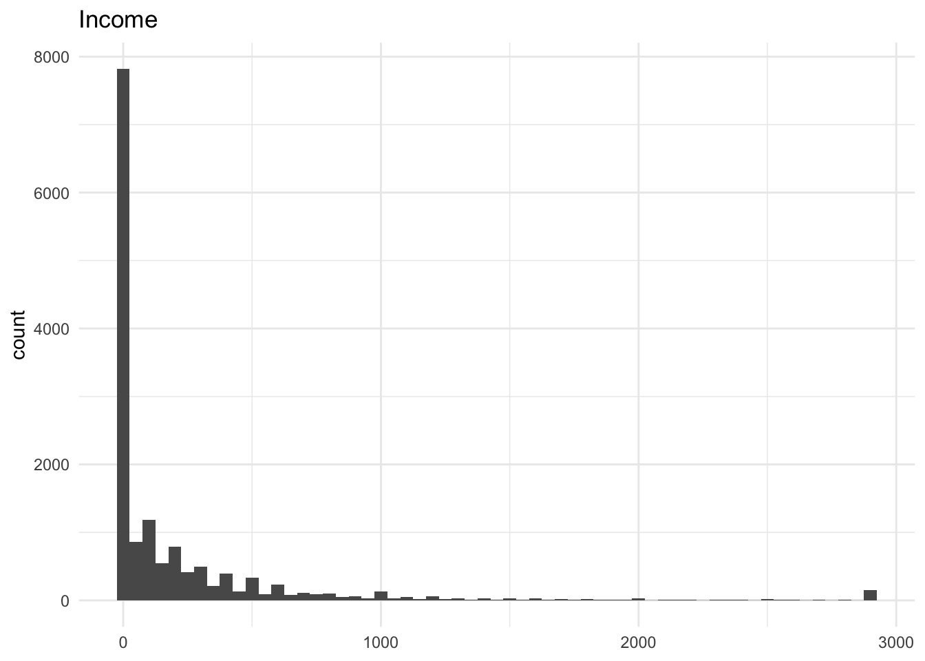
48.8% of total reported income (at the period level) is 0 so I use it as a benchmark to evaluate the different volatility measures.
The period-to-period percent change is missing 7012 out out of 12593 (56%) times.
The period-to-period log percentage change is missing 9194 out of 12593 (73%) times.
The period-to-period arc percentage change is missing 780 out of 12593 (6%) times.
The period-to-period normalized deviation is missing 710 out of 12593 (5.6%) times.
These translate into household-level missingness for the different measures. However, the aggregations often drop missing observations for a household (i.e. median or mean simply ignore missing values).
This translates to:
Code
```{r}#| message: false#| warning: false# For all the measures, compute the number of missing values for income variablemeasures <- c( "sd_log_chg" = "SD Log Change", "mdpct_chg" = "Median % Change", "mean_nchange" = "Mean Normalized Change", "cv" = "Coefficient of Variation", "sd_arc_chg" = "SD Arc Change", "mean_arc_chg" = "Mean Abs Arc Change", "mean_normdev" = "Normalized Deviation", "frac_swing" = "Fraction Large Changes")missing_counts <- sapply(names(measures), function(measure) { sum(is.na(volatility[[paste0(measure, "_income")]]))})# display as a tabledata.frame( Measure = unname(measures), Missing_Count = missing_counts) %>% mutate(Percentage = (Missing_Count / 2272) * 100) %>% kable() %>% kable_styling()```
Measure
Missing_Count
Percentage
sd_log_chg
SD Log Change
1336
58.802817
mdpct_chg
Median % Change
271
11.927817
mean_nchange
Mean Normalized Change
138
6.073944
cv
Coefficient of Variation
118
5.193662
sd_arc_chg
SD Arc Change
56
2.464789
mean_arc_chg
Mean Abs Arc Change
26
1.144366
mean_normdev
Normalized Deviation
0
0.000000
frac_swing
Fraction Large Changes
0
0.000000
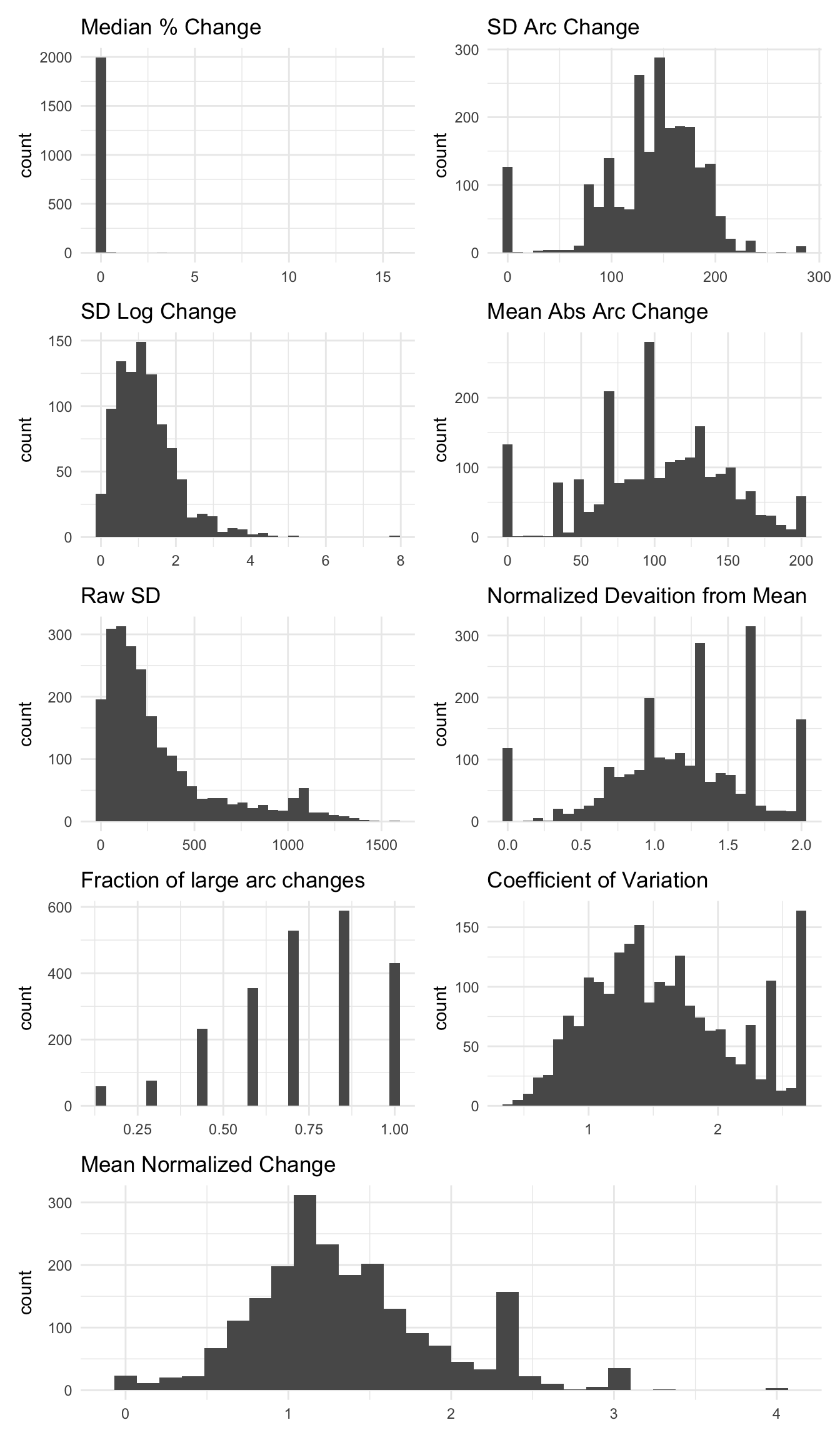
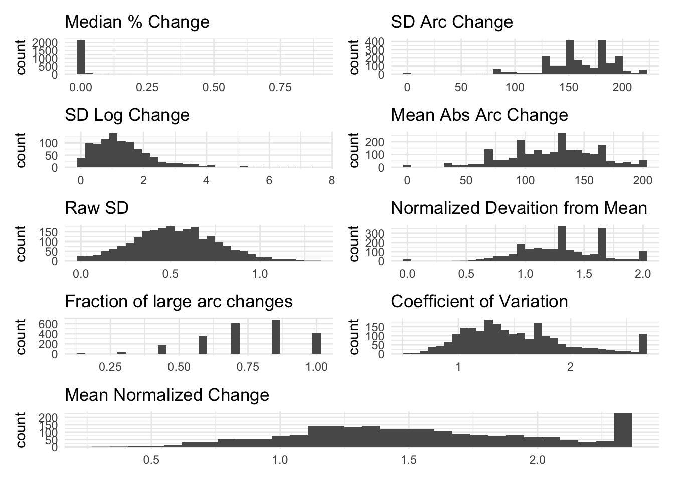
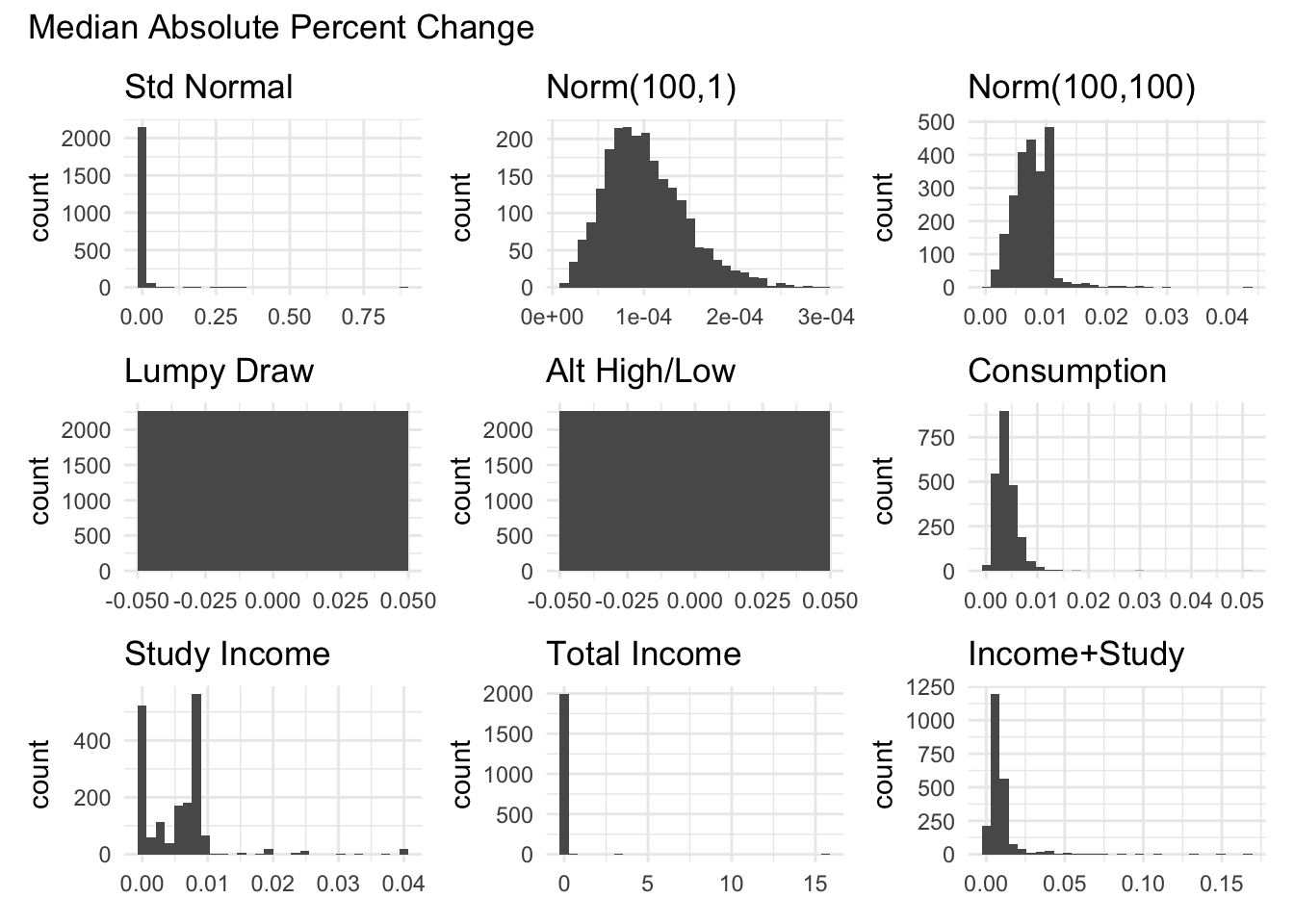
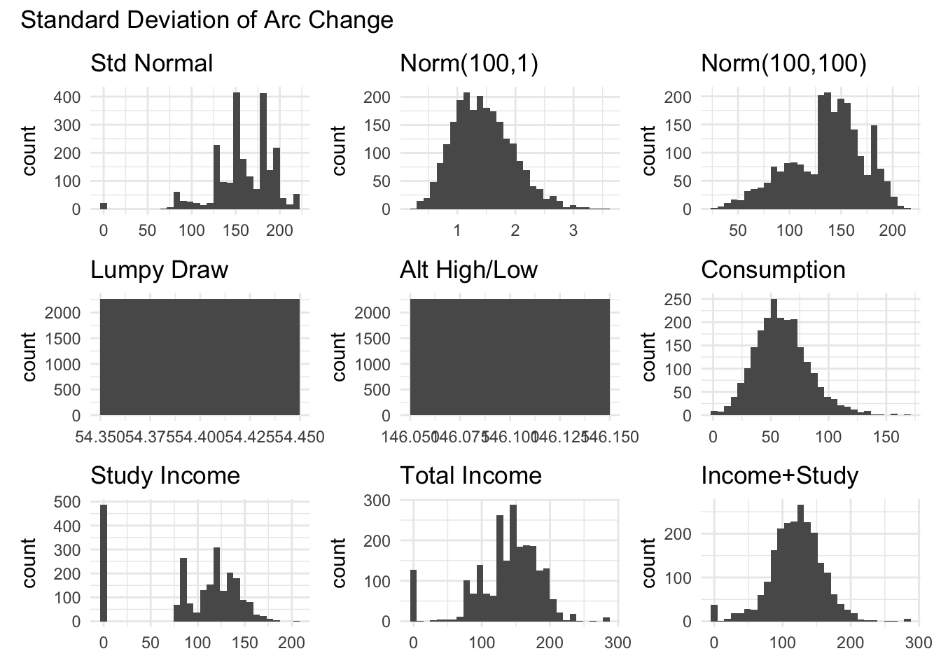
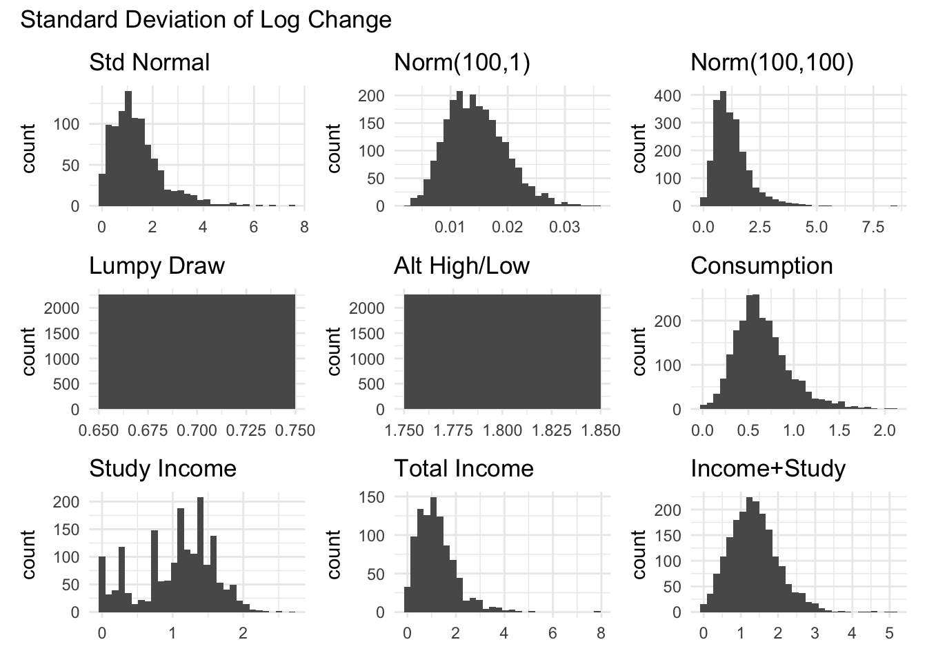
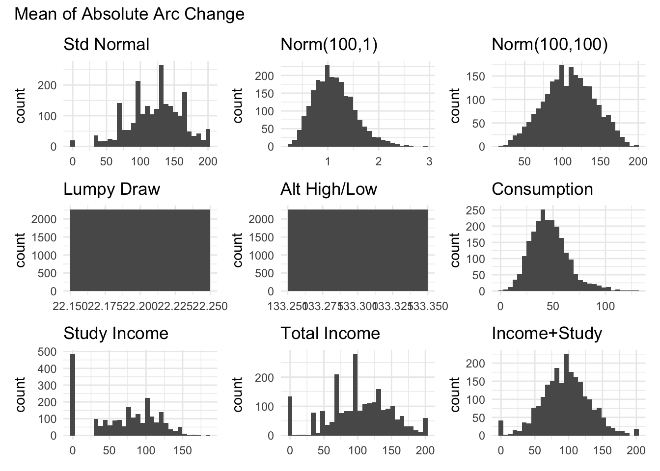
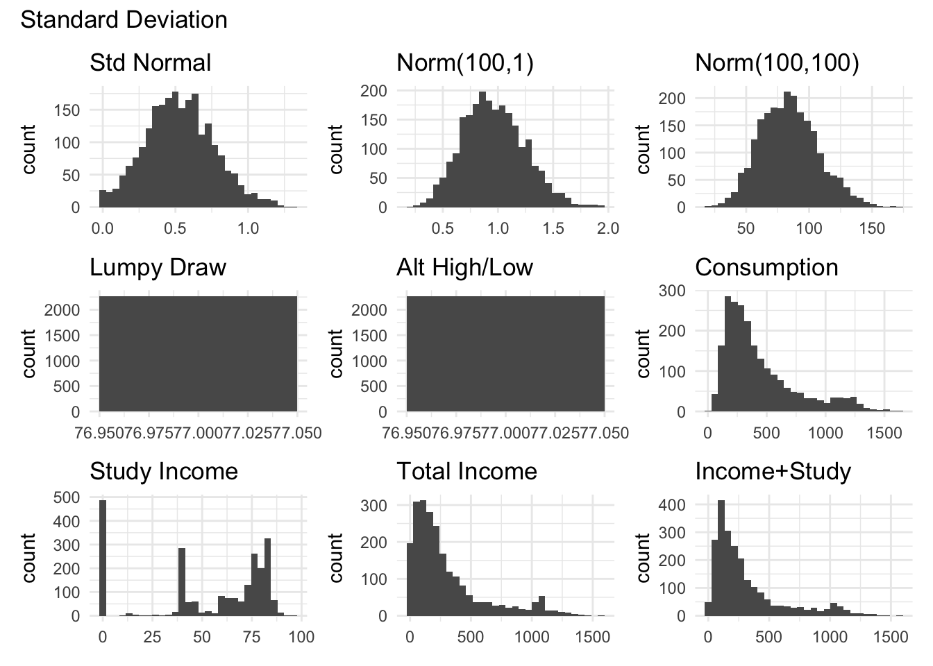
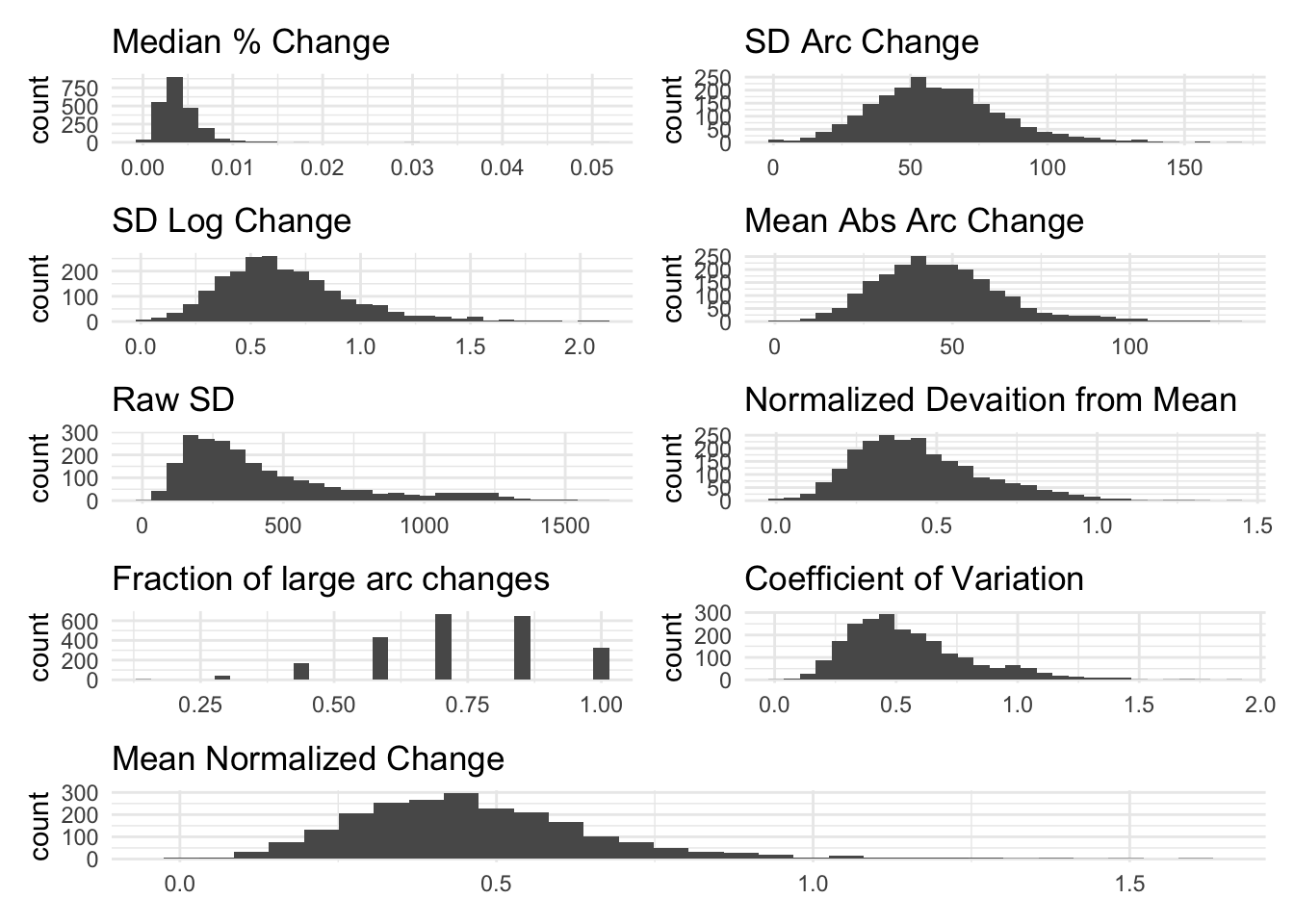
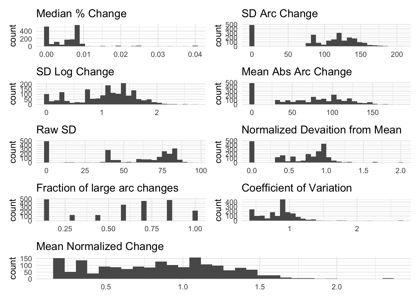
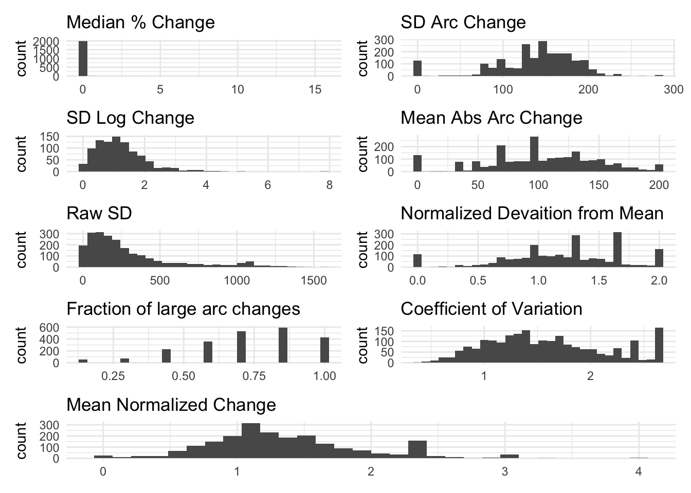
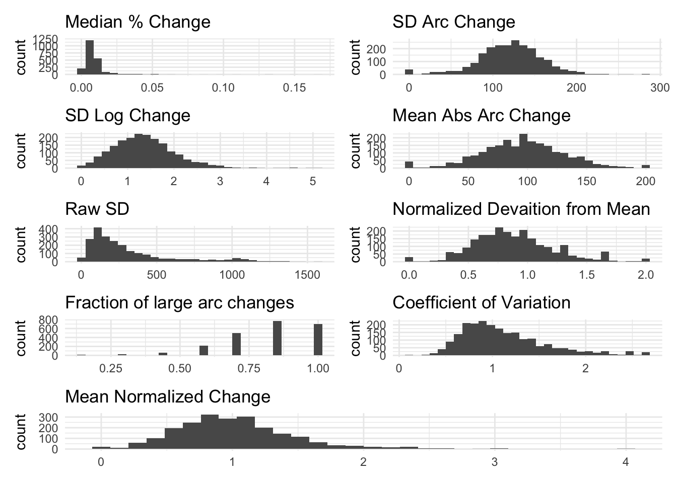
The graphs below show the distributions of the different measures for total income.
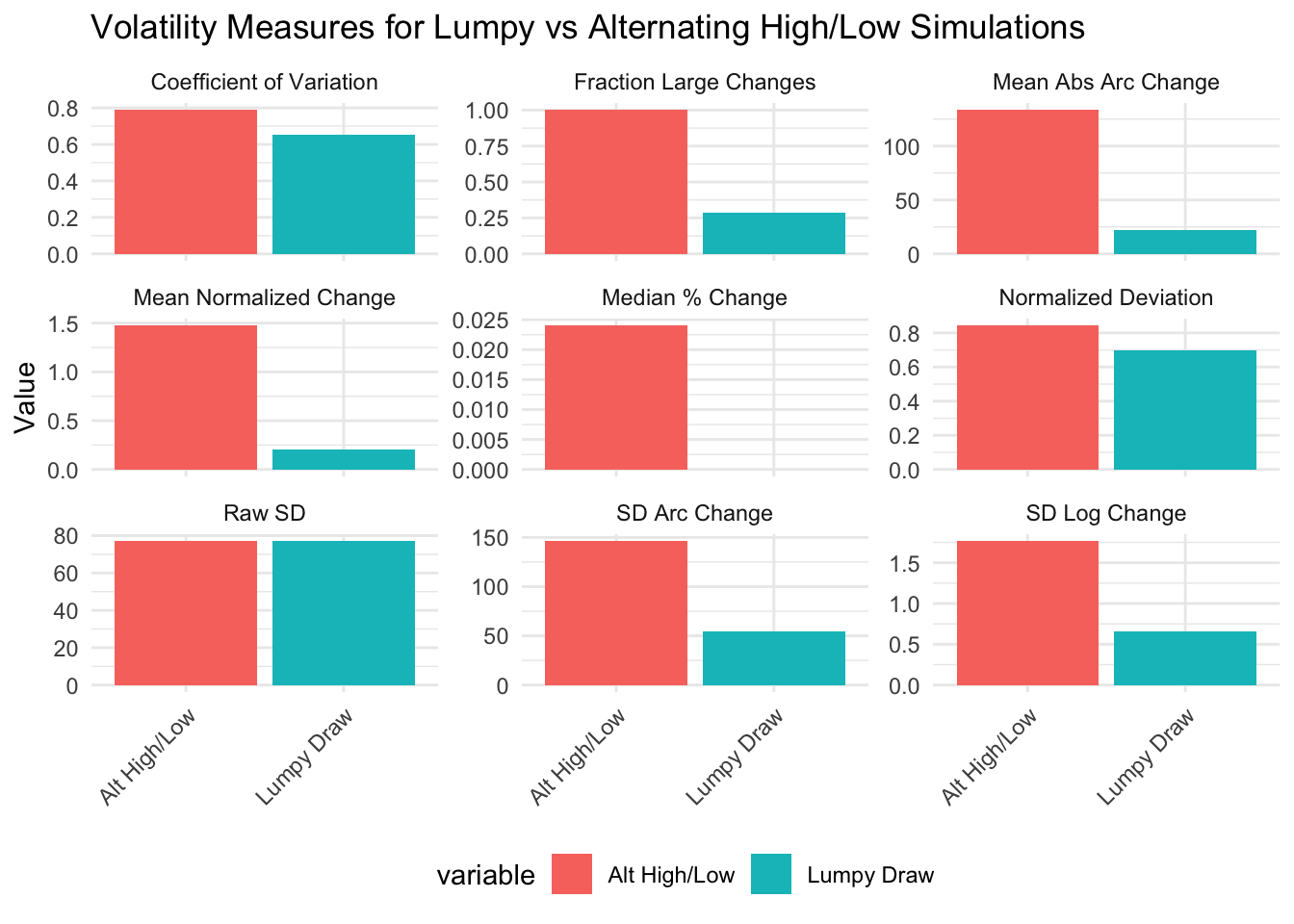
Do they distinguish between lumpy volatility or not?
Code
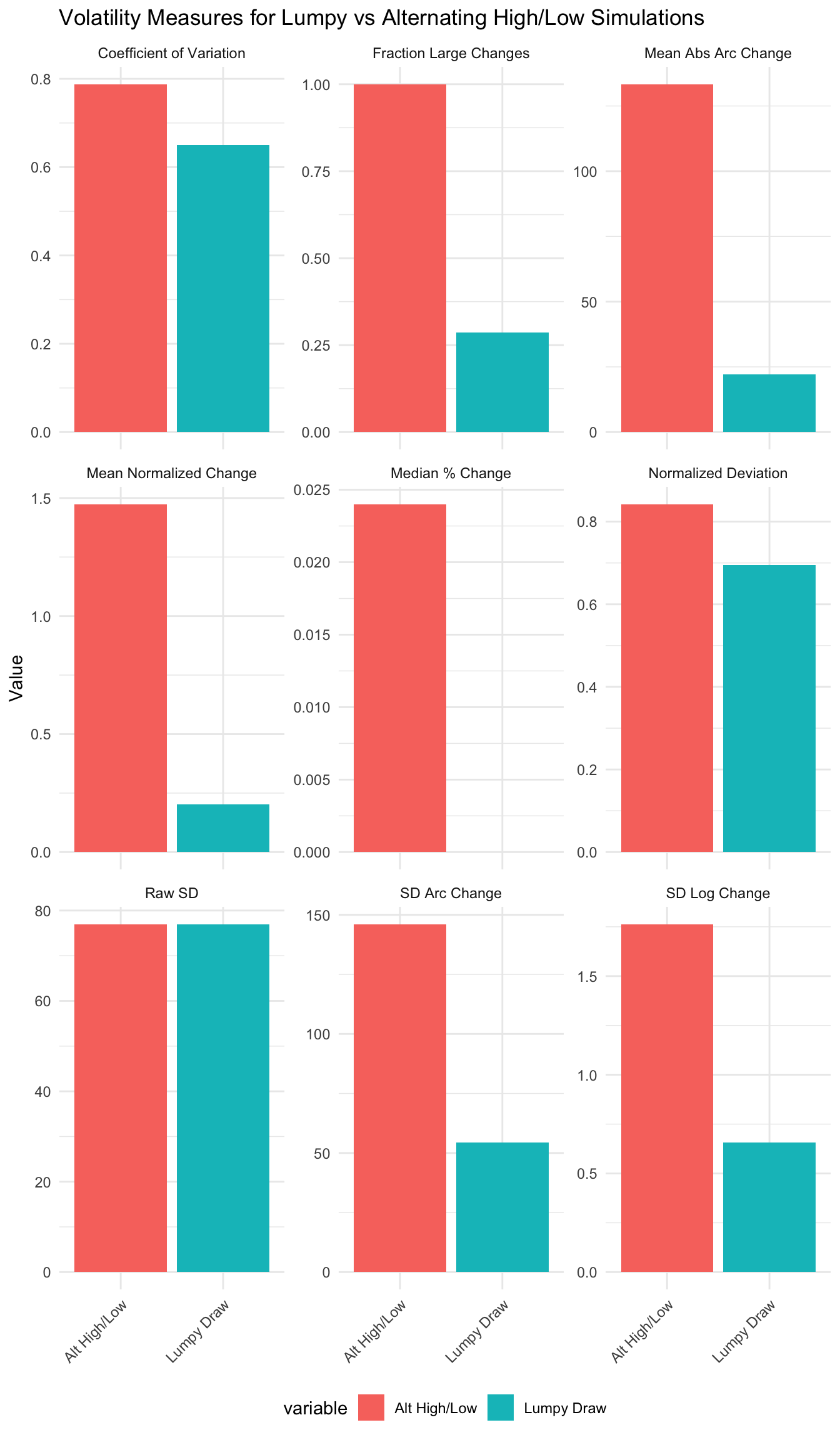
```{r}#| message: false#| warning: false#| fig.height: 12# For all the measures, all the HHs will have exactly the same "volatility" measures since the random values are constant across households. Thus, make a bar graph where the x-axis is the measure and the y-axis is the value. There should be two bars for each variable, lumpy and alternatingmeasures <- c("mdpct_chg" = "Median % Change", "sd_arc_chg" = "SD Arc Change", "sd_log_chg" = "SD Log Change", "mean_arc_chg" = "Mean Abs Arc Change", "sd" = "Raw SD", "mean_normdev" = "Normalized Deviation", "frac_swing" = "Fraction Large Changes", "cv" = "Coefficient of Variation", "mean_nchange" = "Mean Normalized Change")one_row <- volatility %>% slice(1L) %>% select(c(ends_with("simu_lumpy"), ends_with("simu_max_var"))) %>% # pivot long so that each row is a measure-variable combo with a new column indicate the measure pivot_longer(everything(), names_to = "measure_variable", values_to = "value") %>% # Separate measure and variable into two columns mutate(measure = ifelse(grepl("simu_lumpy", measure_variable), sub("_(simu_lumpy)$", "", measure_variable), sub("_(simu_max_var)$", "", measure_variable)), measure = recode(measure, !!!measures), variable = ifelse(grepl("simu_lumpy", measure_variable), "Lumpy Draw", "Alt High/Low")) %>% select(-measure_variable)ggplot(one_row, aes(x=variable, y=value, fill=variable)) + geom_bar(stat="identity") + facet_wrap(~measure, scales="free_y", ncol=3) + labs(title="Volatility Measures for Lumpy vs Alternating High/Low Simulations", x=NULL, y="Value") + theme_minimal() + theme(axis.text.x = element_text(angle = 45, hjust = 1), legend.position = "bottom")```
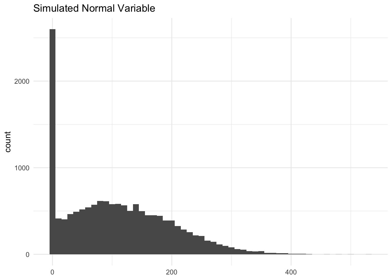
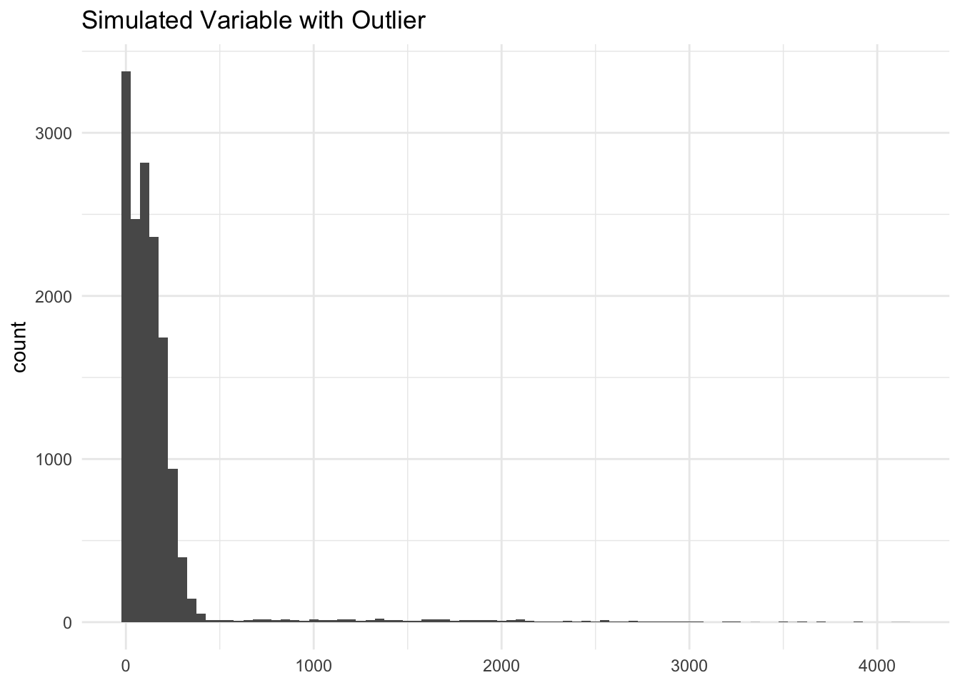
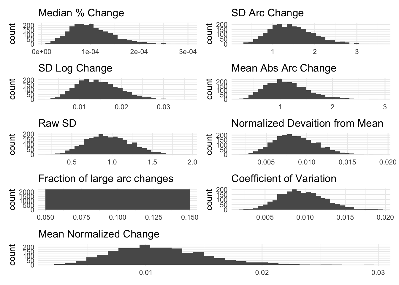
The visualizations below show the distributions of the different volatility measures for a simulated random variable drawn from a normal distribution with mean 100 and standard deviation 100. Values below 0 are bound to 0. Then, I aggregate it to the household level.
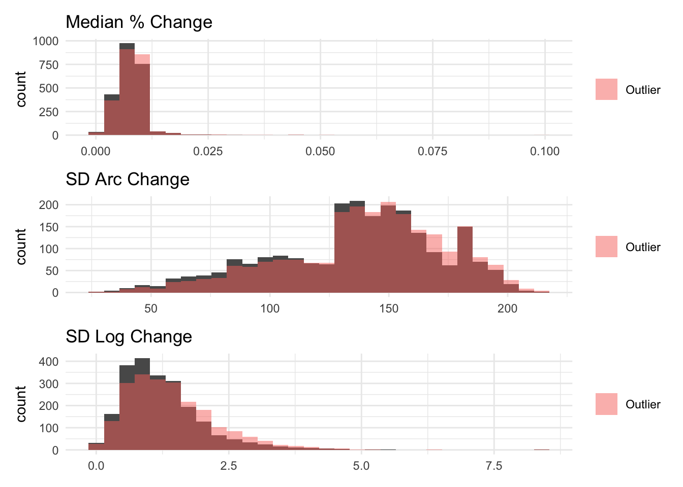
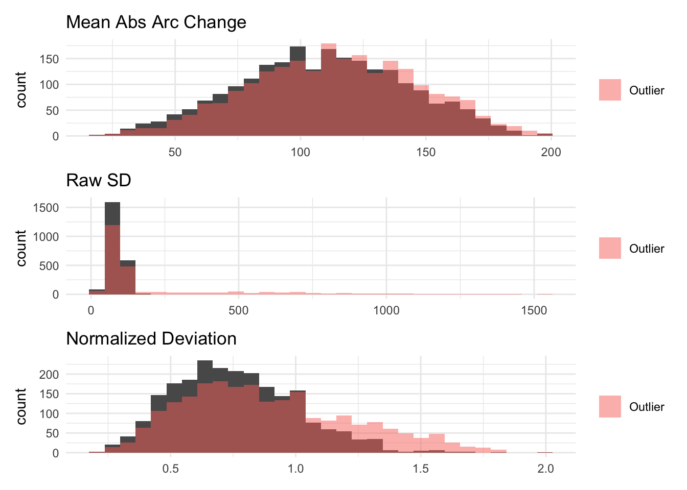
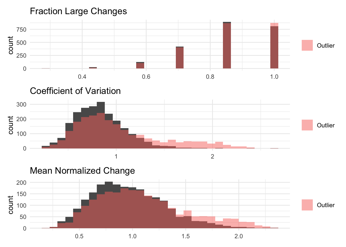
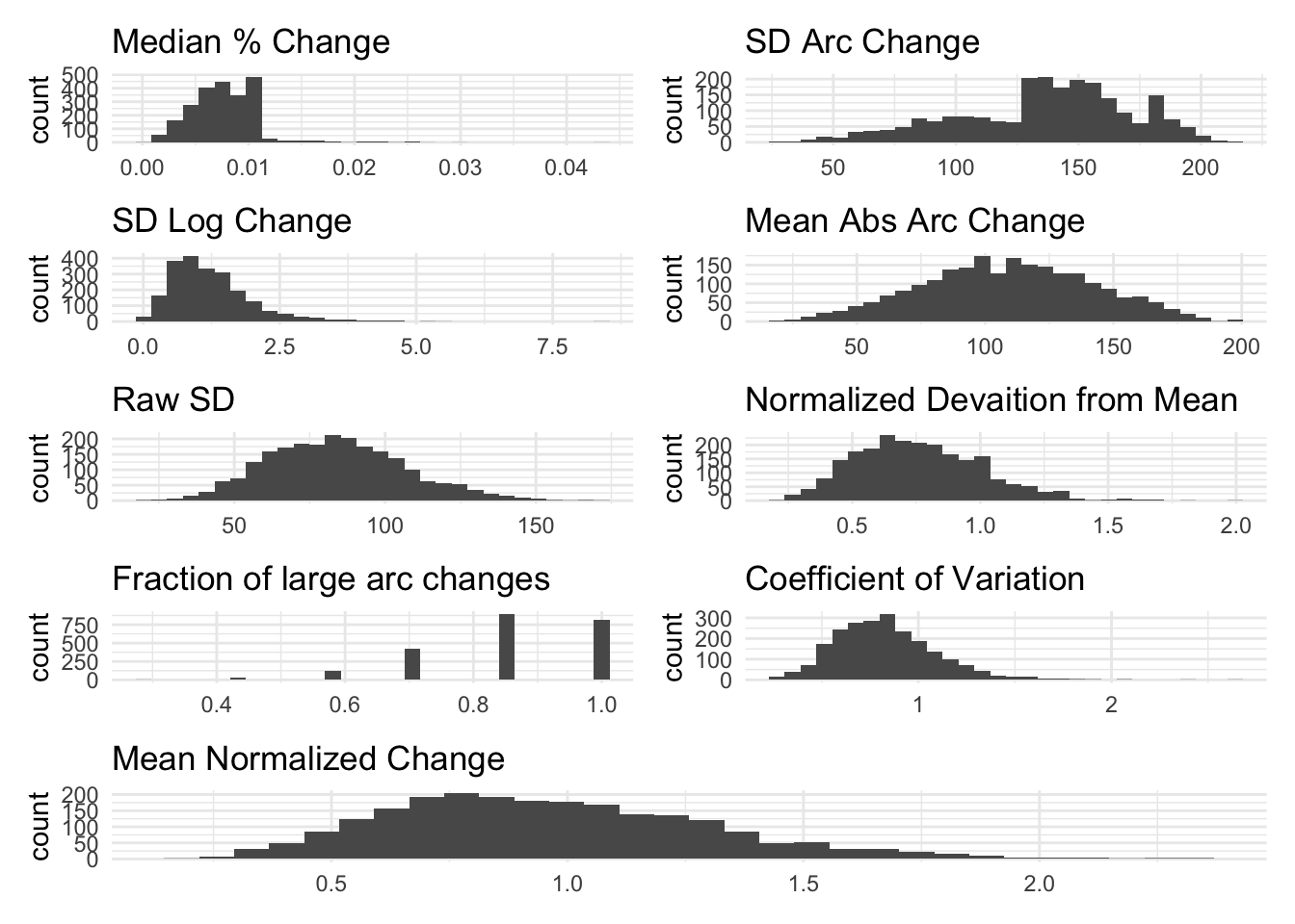
```{r}#| warning: false# For each measure make a p1 + p2 graph where p1 is the measure for simu_nom_hv and p2 is the measure for simu_outlierlumpy_graphs <- imap(measures, ~ volatility %>% ggplot() + geom_histogram(aes(x=.data[[paste0(.y, "_simu_nom_hv")]]), alpha = 1) + geom_histogram(aes(fill = "Outlier", x=.data[[paste0(.y, "_simu_outlier")]]), alpha = 0.5) + labs(title=.x, x=NULL, fill = NULL) + theme_minimal() )# Reduce the first four outlier_comparison into a single patchworks graph by the / operator (stacking)```
The purpose of these figures are to show the different measurements capture (or don’t) time-based volatility (i.e. volatility between P1 and P2) while holding average within-period volatility constant (i.e. overall sum of deviations from the mean is the same)
Code
```{r}#| message: false#| warning: false# For all the measures, all the HHs will have exactly the same "volatility" measures since the random values are constant across households. Thus, make a bar graph where the x-axis is the measure and the y-axis is the value. There should be two bars for each variable, lumpy and alternatingmeasures <- c("mdpct_chg" = "Median % Change", "sd_arc_chg" = "SD Arc Change", "sd_log_chg" = "SD Log Change", "mean_arc_chg" = "Mean Abs Arc Change", "sd" = "Raw SD", "mean_normdev" = "Normalized Deviation", "frac_swing" = "Fraction Large Changes", "cv" = "Coefficient of Variation", "mean_nchange" = "Mean Normalized Change")one_row <- volatility %>% slice(1L) %>% select(c(ends_with("simu_lumpy"), ends_with("simu_max_var"))) %>% # pivot long so that each row is a measure-variable combo with a new column indicate the measure pivot_longer(everything(), names_to = "measure_variable", values_to = "value") %>% # Separate measure and variable into two columns mutate(measure = ifelse(grepl("simu_lumpy", measure_variable), sub("_(simu_lumpy)$", "", measure_variable), sub("_(simu_max_var)$", "", measure_variable)), measure = recode(measure, !!!measures), variable = ifelse(grepl("simu_lumpy", measure_variable), "Lumpy Draw", "Alt High/Low")) %>% select(-measure_variable)ggplot(one_row, aes(x=variable, y=value, fill=variable)) + geom_bar(stat="identity") + facet_wrap(~measure, scales="free_y", ncol=3) + labs(title="Volatility Measures for Lumpy vs Alternating High/Low Simulations", x=NULL, y="Value") + theme_minimal() + theme(axis.text.x = element_text(angle = 45, hjust = 1), legend.position = "bottom")```
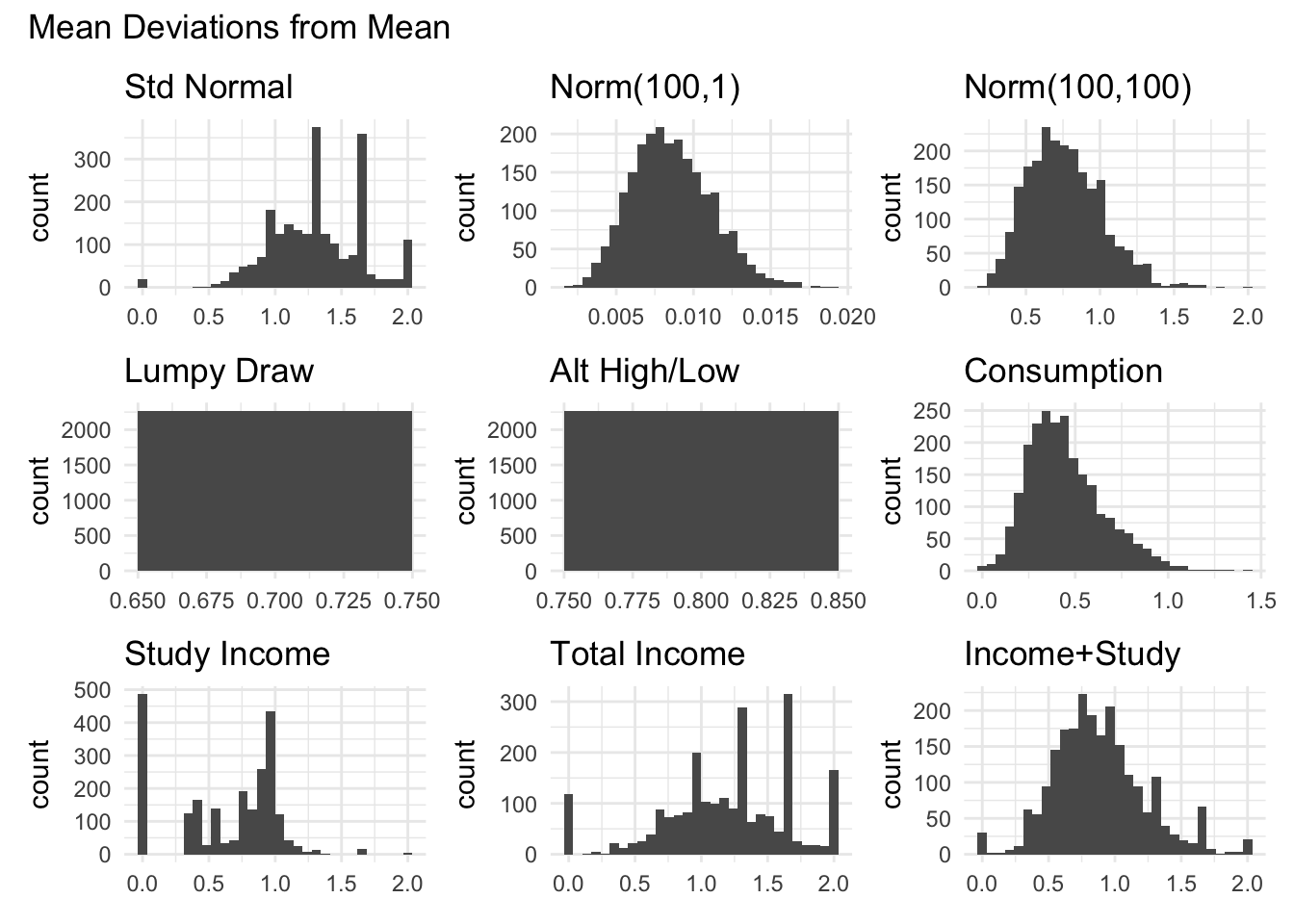
```{r}#| message: false#| warning: falsegraph_all_variables_for_measure("mean_normdev_", "Mean Deviations from Mean")```
Code
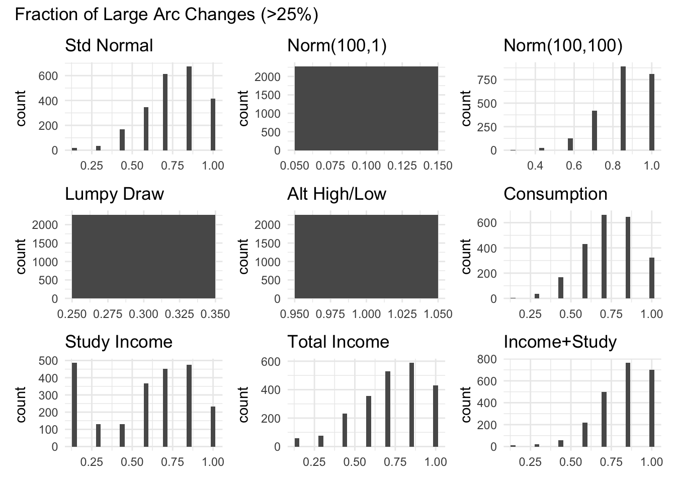
```{r}#| message: false#| warning: falsegraph_all_variables_for_measure("frac_swing_", "Fraction of Large Arc Changes (>25%)")```
Code
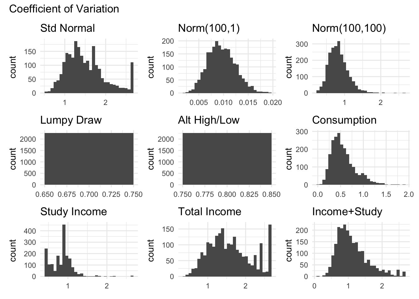
```{r}#| message: false#| warning: falsegraph_all_variables_for_measure("cv_", "Coefficient of Variation")```
Code
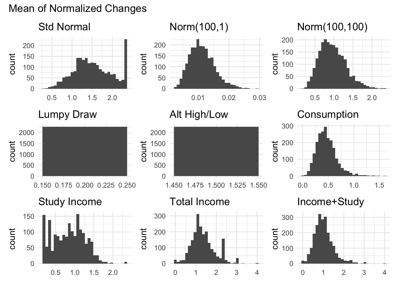
```{r}#| message: false#| warning: falsegraph_all_variables_for_measure("mean_nchange_", "Mean of Normalized Changes")```
The fraction of large changes is too discrete given the short amount of periods which limit the number of values (7) it can take on
The raw standard deviation has a large tail, suggesting that it would be very sensitive to outliers. Additionally, it seems to “swallow” some variation as the Total Income and total income + study income distributions are very similar. This is surprising given that a lot of the other measures show large differences between these two variables.
The coefficient of variation normalizes the standard deviation by the mean, which can help compare volatility across variables with different scales. However, it is undefined when the mean is zero and can be problematic with variables that have values near zero.
The mean of normalized changes measures period-to-period changes scaled by the household mean, capturing volatility relative to average levels while handling zero values better than log or percent changes.
Real Variables
Below, we visualize the volatility measures for outcomes from our study
Brewer, Mike, Nye Cominetti, and Stephen P. Jenkins. 2025. “What Do We Know about Income and Earnings Volatility?”Review of Income and Wealth 71 (2): e70013. https://doi.org/10.1111/roiw.70013.
Ganong, Peter, Pascal Noel, Christina Patterson, Joseph Vavra, and Alexander Weinberg. 2025. Earnings Instability. w34227. Cambridge, MA: National Bureau of Economic Research. https://doi.org/10.3386/w34227.