March 10, 2026 - Analysis Wk.2: CDFs

Published

March 10, 2026

Abstract

CDFs that compare outcomes between arms

Discussed on March 3, 2026. Meeting notes available here.

Big Takeaways:

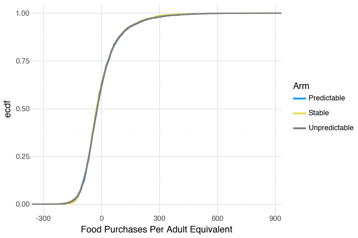
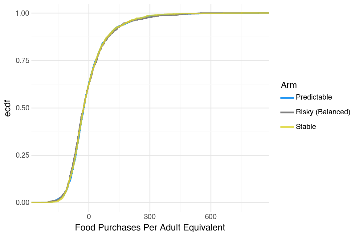
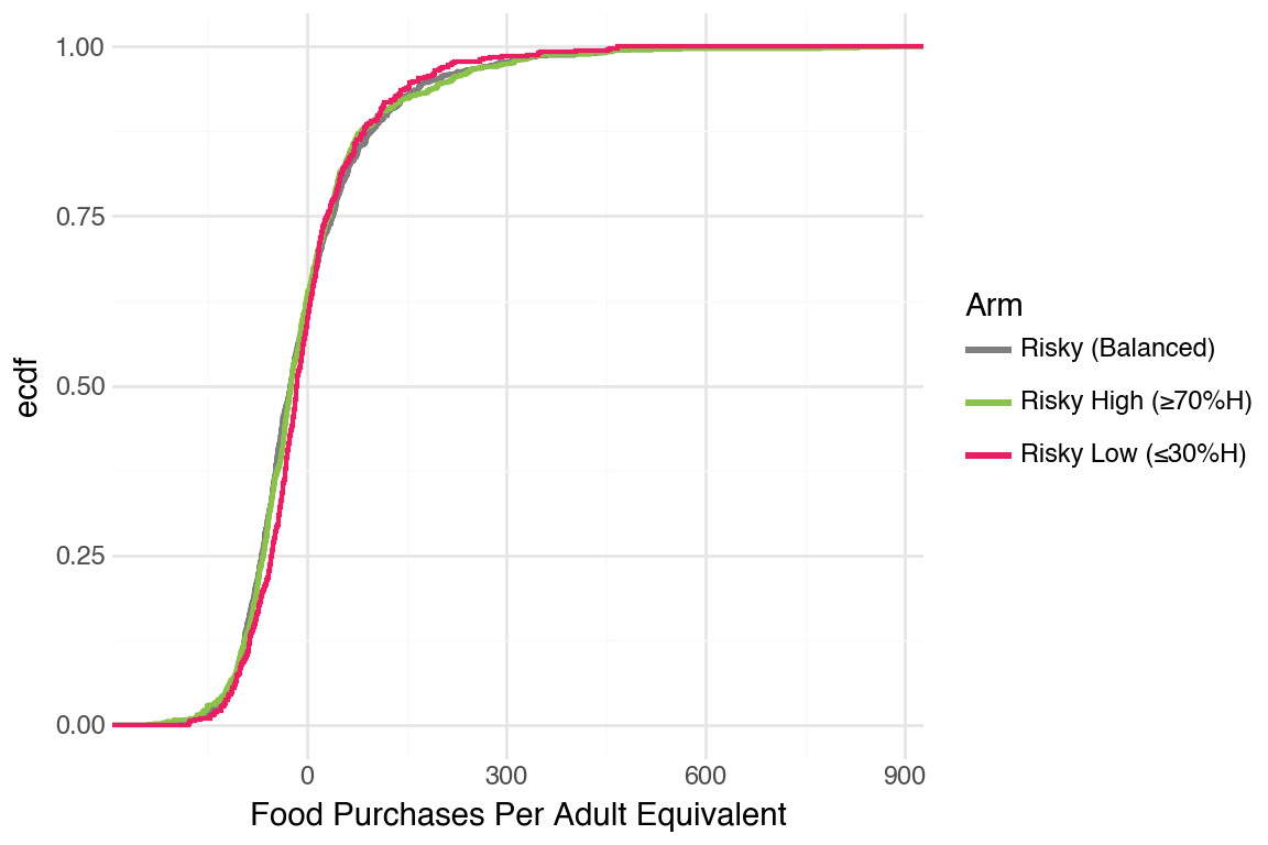
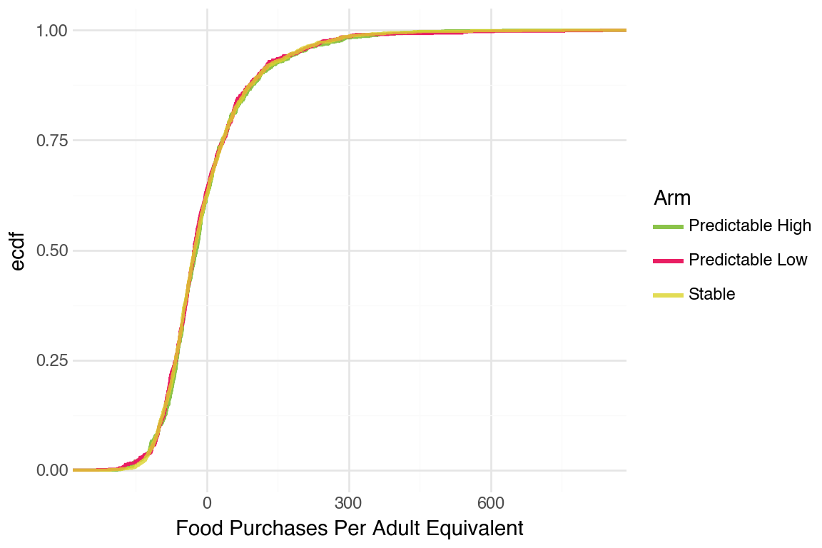
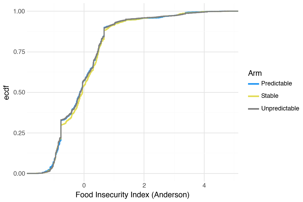
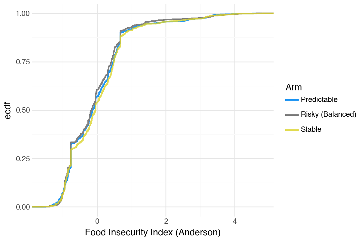
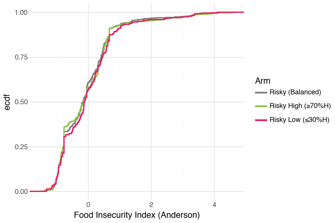
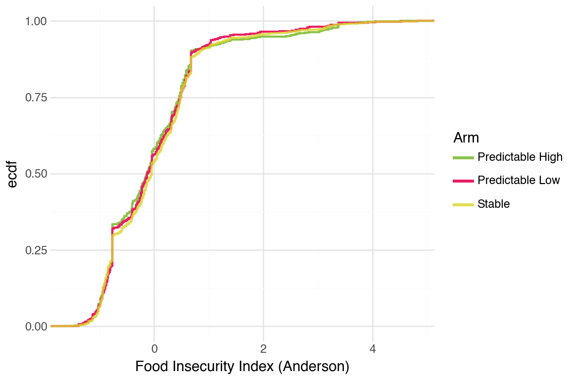
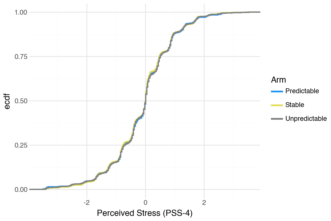
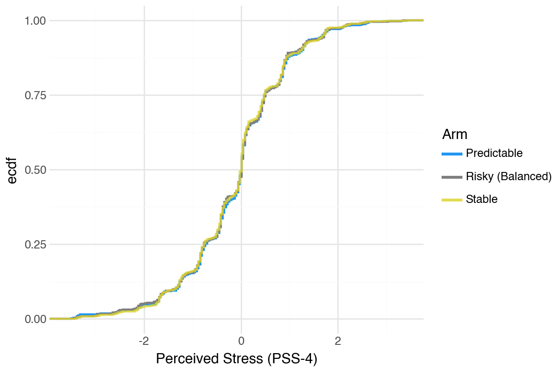
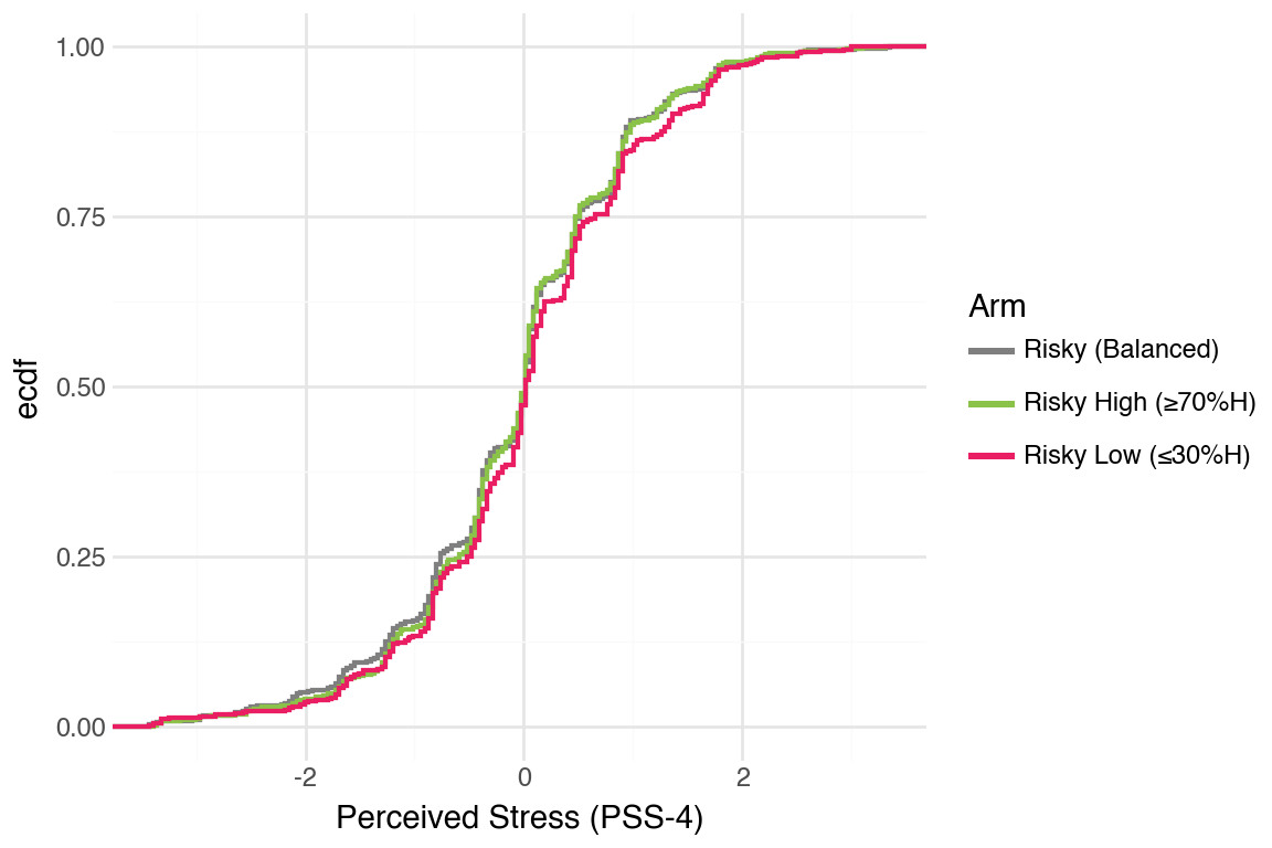
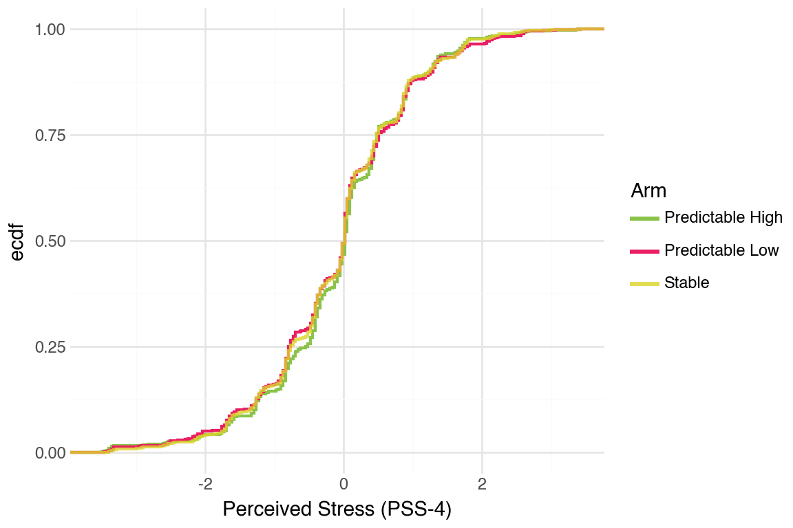
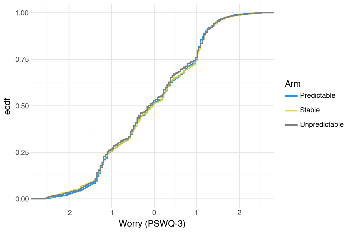
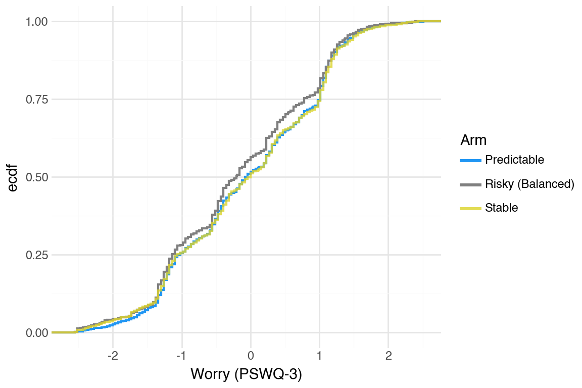
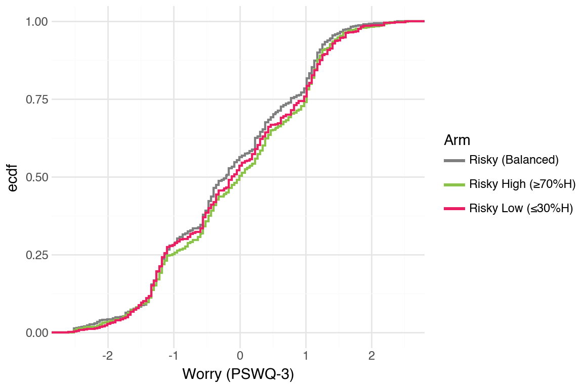
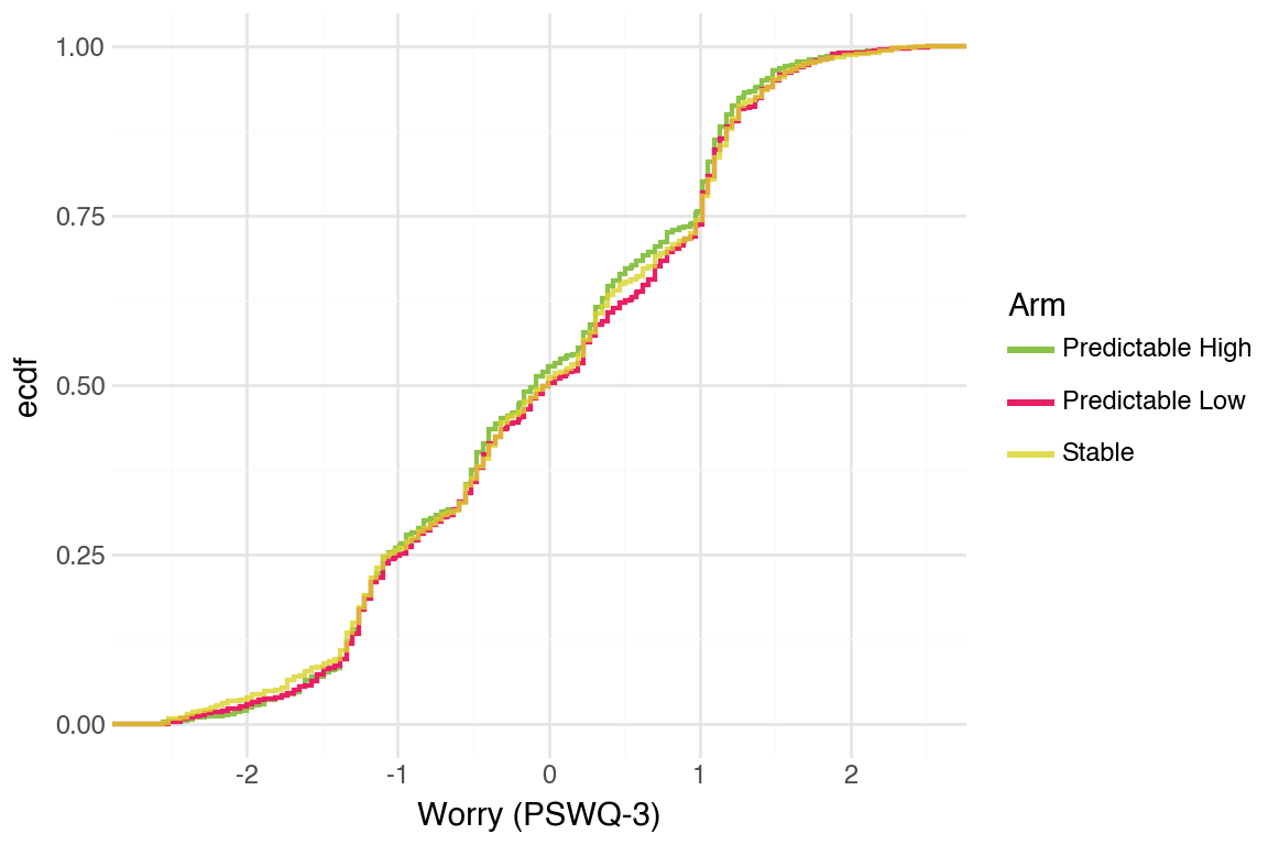
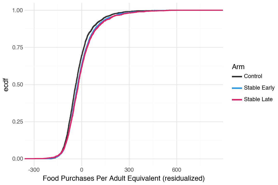
  • CDFs were hard to tell apart. One pattern that was noticeable was that Stable arm did better than the others.
  • People smoothed food purchases very well. We decided to take a look at the adult equivalent version to see if that revealed more differences between arms.
    • We also decided to take a look at debt to see if that was a reasonable source of consumption smoothing or sink of people spending their money

Analysis for this week:

  • Generate CDFs for the adult equivalent version of food purchases (no noticeable difference)
  • Generate CDFs for other mental health outcomes (PSS-4, PSWQ-3); separation is even smaller compared to the PHQ and GAD
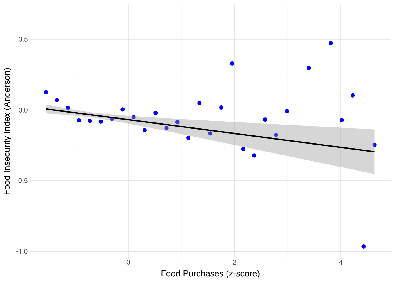
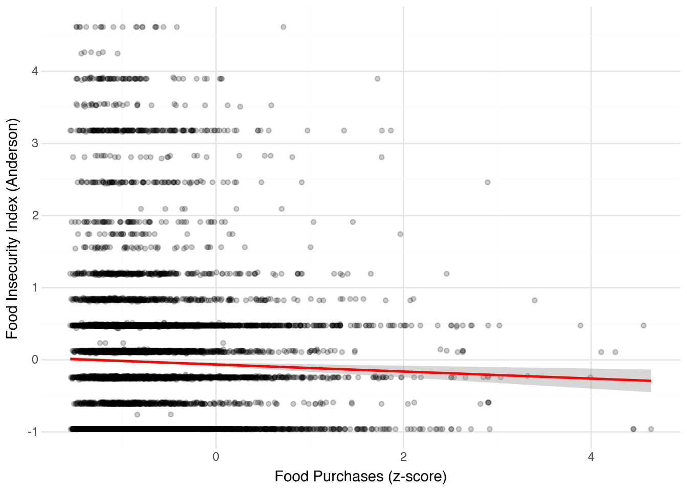
  • Correlation between food insecurity and food purchases: yes there is a correlation in the degree we expect. However, it is not too strong
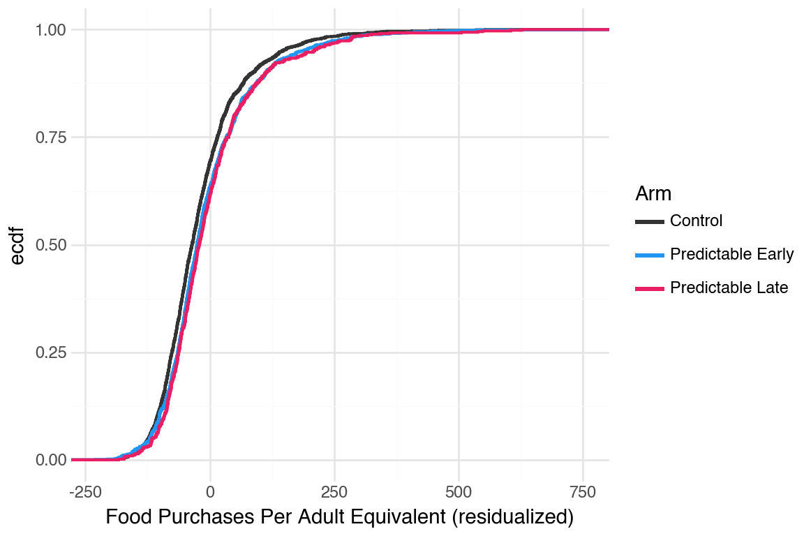
  • Survey timing doesn’t seem to make much of a difference: late and early predictable look similar in their food purchase decisions
Code
```{python}
#| label: df-subseting
phone_survey_panel = panel_df[(panel_df["period"] > 0) & (panel_df["period"] < 6) & (panel_df["treatment"] != 0)].copy()
phone_survey_panel_w_control = panel_df[(panel_df["period"] > 0) & (panel_df["period"] < 6)].copy()

balanced_only_ph = phone_survey_panel[phone_survey_panel["treatment_balanced"].isin([1, 2, 3])].copy() 
balanced_only_ph_w_control = phone_survey_panel_w_control[phone_survey_panel_w_control["treatment_balanced"].isin([1, 2, 3])].copy()

risky_only = phone_survey_panel[phone_survey_panel["treatment"].isin([3, 4, 5])].copy()
risky_only_w_control = phone_survey_panel_w_control[phone_survey_panel_w_control["treatment"].isin([3, 4, 5])].copy()
```

CDFs

Note

All outcomes shown below are residualized on baseline values of the outcome. See appendix for non-residualized CDFs.

Food Purchases

Code
```{python}
make_cdf(phone_survey_panel, "food_purchase_total_99_ae_resid", "arm", None)
```

Code
```{python}
make_cdf(balanced_only_ph, "food_purchase_total_99_ae_resid", "arm_split", None)
```

Code
```{python}
make_cdf(risky_only, "food_purchase_total_99_ae_resid", "arm_split", None)
```

Code
```{python}
make_cdf(phone_survey_panel, "food_purchase_total_99_ae_resid", "arm_pred_split", None)
```

Food Insecurity Index (Anderson)

Code
```{python}
make_cdf(phone_survey_panel, "fi_index_anderson_resid", "arm", None)
```

Code
```{python}
make_cdf(balanced_only_ph, "fi_index_anderson_resid", "arm_split", None)
```

Code
```{python}
make_cdf(risky_only, "fi_index_anderson_resid", "arm_split", None)
```

Code
```{python}
make_cdf(phone_survey_panel, "fi_index_anderson_resid", "arm_pred_split", None)
```

PSS-4

Code
```{python}
make_cdf(phone_survey_panel, "pss4_z_resid", "arm", None)
```

Code
```{python}
make_cdf(balanced_only_ph, "pss4_z_resid", "arm_split", None)
```

Code
```{python}
make_cdf(risky_only, "pss4_z_resid", "arm_split", None)
```

Code
```{python}
make_cdf(phone_survey_panel, "pss4_z_resid", "arm_pred_split", None)
```

PSWQ-3

Code
```{python}
make_cdf(phone_survey_panel, "pswq3_z_resid", "arm", None)
```

Code
```{python}
make_cdf(balanced_only_ph, "pswq3_z_resid", "arm_split", None)
```

Code
```{python}
make_cdf(risky_only, "pswq3_z_resid", "arm_split", None)
```

Code
```{python}
make_cdf(phone_survey_panel, "pswq3_z_resid", "arm_pred_split", None)
```

Code
```{python}
# Generate a df with the following columns:
# - outcome
# - arm column
# - KS p-value (permutation)
# - KS p-value (asymptotic)
# - AD p-value (permutation)
# - AD p-value (asymptotic)
outcomes_to_test = [
    "food_purchase_total_99_ae_resid",
    "fi_index_anderson_resid",
    "pss4_z_resid",
    "pswq3_z_resid",
    "phq2_z_resid",
    "gad2_z_resid",
]

arm_columns = ["arm", "arm_split"]

records = []
for outcome in outcomes_to_test:
    for arm_col in arm_columns:
        res = clustered_permutation_test(phone_survey_panel, outcome, arm_col)
        records.append({
            "outcome": outcome,
            "arm_col": arm_col,
            "ks_stats": {pair: vals["stat"] for pair, vals in res["ks"].items()},
            "ks_p_perm": {pair: vals["p_value"] for pair, vals in res["ks"].items()},
            "ks_p_asymp": {pair: vals["p_value_asymptotic"] for pair, vals in res["ks"].items()},
        })
records_df = pd.DataFrame(records)
```

Kolmogorov-Smirnov Test

The table below display’s two values. The asymptotic p-value is the one we would get from a standard KS test that doesn’t account for clustering. The permutation p-value generated by shuffling treatment labels at the household level and calculating the KS test statistic for each shuffle. The permutation p-value is then the proportion of shuffles where the KS stat is as extreme or more extreme than the observed distribution generated through the shuffle-then-calculate approach.

Code
```{python}
# Explode the nested dict columns into one row per arm pair

ARM_COL_LABELS  = {"arm": "3-Arm (S/P/U)", "arm_split": "4-Arm Split"}
OUTCOME_LABELS  = {f"{k}_resid": v for k, v in outcomes.items()}

def sig_stars(p):
    if p < 0.01:  return "***"
    if p < 0.05:  return "**"
    if p < 0.10:  return "*"
    return ""


ks_rows = []
for _, row in records_df.iterrows():
    for pair, stat in row["ks_stats"].items():
        arm_a, arm_b = pair
        ks_rows.append({
            "Outcome":      OUTCOME_LABELS.get(row["outcome"], row["outcome"]),
            "Arm A":        arm_a,
            "Arm B":        arm_b,
            "p (Clustered Perm.)": row["ks_p_perm"][pair],
            "p (Asymptotic)":      row["ks_p_asymp"][pair],
        })

ks_table = pd.DataFrame(ks_rows)
ks_table["Sig."]        = ks_table["p (Clustered Perm.)"].apply(sig_stars)
ks_table = ks_table.reset_index(drop=True)
ojs_define(data=ks_table.to_dict(orient="records"))
```
Code
```{ojs}
//| label: ks-table-interactive
//| panel: input
viewof filtered_outcome = Inputs.select(
    ["All Outcomes"].concat(Array.from(new Set(data.map(d => d.Outcome)))),
    {label: "Filter by Outcome:"}
)

filtered_data = filtered_outcome === "All Outcomes" 
    ? data 
    : data.filter(d => d.Outcome === filtered_outcome)

Inputs.table(filtered_data, {
    rows: 15,
    maxWidth: 800,
    multiple: false,
    layout: "auto"
})
```

Correlation between Food Insecurity and Food Purchases

Code
```{python}
(
    ggplot(phone_survey_panel_w_control, aes(y="fi_index_anderson", x='food_purchase_total_99_ae_z')) 
    #+ geom_point(alpha=0.2) 
    + stat_summary_bin(
        bins=30, 
        geom="point", 
        color="blue", 
        size=2
    )
    + geom_smooth(method="lm")
    + theme_minimal()
    + labs(x="Food Purchases (z-score)", y="Food Insecurity Index (Anderson)")
)
```

Code
```{python}
(
    ggplot(phone_survey_panel_w_control, aes(y="fi_index_anderson", x='food_purchase_total_99_ae_z')) 
    + geom_point(alpha=0.2) 
    + geom_smooth(method="lm", color="red")
    + theme_minimal()
    + labs(x="Food Purchases (z-score)", y="Food Insecurity Index (Anderson)")
)
```

Debt Summary Stats

Code
```{python}
#| label: debt-data-prep
debt["loan_source"] = debt["loan_source"].astype(str)
debt["period"] = debt["period"].astype(str)
debt["loan_amount_total_99"] = debt["loan_amount_total"].clip(upper=99)
debt_no_endline = debt[debt["period"] != 6].copy()
```

Count of Loans by Source

The average borrowed amount is around 95 cedis. The average within sources doesn’t vary much and ranges from 80-100 cedis.

Code
```{python}
#| label: debt-count-by-source
source_counts = (
    debt_no_endline
    .groupby("loan_source", as_index=False)
    .size()
    .rename(columns={"size": "count"})
    .sort_values("count", ascending=False)
)

(
    ggplot(source_counts, aes(x="reorder(loan_source, count)", y="count"))
    + geom_col(fill="#2196F3")
    + geom_text(aes(label="count"), ha="left", nudge_y=5, size=8)
    + coord_flip()
    + theme_minimal()
    + labs(x="Loan Source", y="Number of Loans", title="Count of Loans by Source")
    + theme(figure_size=(7, 5))
)
```

Code
```{python}
#| label: debt-count-by-period
source_counts_period = (
    debt_no_endline
    .groupby("period", as_index=False)
    .size()
    .rename(columns={"size": "count"})
    .sort_values("count", ascending=False)
)

(
    ggplot(source_counts_period, aes(x="period", y="count"))
    + geom_col(fill="#2196F3")
    + geom_text(aes(label="count"), ha="left", nudge_y=10, size=8)
    + theme_minimal()
    + labs(x="Period", y="Number of Loans")
    + theme(figure_size=(7, 5))
)
```

Code
```{python}
#| label: debt-count-by-source-period
source_period_counts = (
    debt_no_endline
    .groupby(["period", "loan_source"], as_index=False)
    .size()
    .rename(columns={"size": "count"})
)

# Order sources by overall count (descending)
source_order = source_counts["loan_source"].tolist()
source_period_counts["loan_source"] = pd.Categorical(
    source_period_counts["loan_source"], categories=source_order, ordered=True
)

(
    ggplot(source_period_counts, aes(x="loan_source", y="count", fill="period"))
    + geom_col(position="dodge")
    + coord_flip()
    + theme_bw()
    + labs(x="Loan Source", y="Number of Loans", title="Count of Loans by Source and Period")
    + theme(
        figure_size=(8, 6),
        axis_text_x=element_text(size=8),
        legend_position="right",
    )
    + scale_fill_brewer(type="qual", palette="Set2", name="Period")
)
```

Counts by Arm

Code
```{python}
#| label: debt-count-by-period-arm
source_counts_period_arm = (
    debt
    .groupby(["period", "treatment"], as_index=False, observed=True)
    .size()
    .rename(columns={"size": "count"})
)

# Add within-period percentage
period_totals = source_counts_period_arm.groupby("period")["count"].transform("sum")
source_counts_period_arm["pct"] = (source_counts_period_arm["count"] / period_totals * 100).round(1)

# Map treatment to labels
source_counts_period_arm["arm"] = source_counts_period_arm["treatment"].map(TREATMENT_LABELS).fillna(
    source_counts_period_arm["treatment"].astype(str)
)

# Pivot to wide: rows = period, columns = arm, cells = "N (X%)"
source_counts_period_arm["cell"] = (
    source_counts_period_arm["count"].astype(str)
    + " ("
    + source_counts_period_arm["pct"].astype(str)
    + "%)"
)

arm_order = ["Control", "Stable", "Predictable", "Risky"]
pivot = (
    source_counts_period_arm
    .pivot(index="period", columns="arm", values="cell")
    .reindex(columns=[a for a in arm_order if a in source_counts_period_arm["arm"].unique()])
    .reset_index()
    .rename(columns={"period": "Period"})
)

# Add row totals
period_total_counts = source_counts_period_arm.groupby("period")["count"].sum().reset_index().rename(columns={"count": "Total"})
pivot = pivot.merge(period_total_counts.rename(columns={"period": "Period"}), on="Period")
# Set period as the index for pretty printing
pivot = pivot.set_index("Period")
pivot
```
Control Stable Predictable Risky Total
Period
0 217 (17.1%) 214 (16.9%) 240 (18.9%) 596 (47.0%) 1267
1 88 (15.6%) 102 (18.1%) 107 (19.0%) 266 (47.2%) 563
2 80 (15.4%) 73 (14.0%) 114 (21.9%) 253 (48.7%) 520
3 80 (17.9%) 74 (16.6%) 81 (18.2%) 211 (47.3%) 446
4 50 (12.9%) 67 (17.3%) 77 (19.8%) 194 (50.0%) 388
5 63 (16.1%) 71 (18.1%) 70 (17.9%) 188 (48.0%) 392
6 192 (15.8%) 253 (20.8%) 225 (18.5%) 546 (44.9%) 1216
Code
```{python}
#| label: debt-purpose-prep
purpose_counts = (
    debt
    .groupby(["loan_purpose", "period"], as_index=False, observed=True)
    .size()
    .rename(columns={"size": "count"})
    .sort_values("count", ascending=False)
)

purpose_order = purpose_counts["loan_purpose"].tolist()
```

Count of Loans by Purpose

Code
```{python}
#| label: debt-count-by-purpose

bl_purpose_counts = purpose_counts[purpose_counts["period"] <= "0"].copy()
(
    ggplot(bl_purpose_counts, aes(x="reorder(loan_purpose, count)", y="count"))
    + geom_col(fill="#2196F3")
    + geom_text(aes(label="count"), ha="left", nudge_y=3, size=8)
    + coord_flip()
    + theme_minimal()
    + labs(x="Loan Purpose", y="Number of Loans", title="Count of Loans by Purpose")
    + theme(figure_size=(7, 5))
)
```

Code
```{python}
#| label: debt-count-by-purpose-endline

el_purpose_counts = purpose_counts[purpose_counts["period"] == "6"].copy()

(
    ggplot(el_purpose_counts, aes(x="reorder(loan_purpose, count)", y="count"))
    + geom_col(fill="#2196F3")
    + geom_text(aes(label="count"), ha="left", nudge_y=3, size=8)
    + coord_flip()
    + theme_minimal()
    + labs(x="Loan Purpose", y="Number of Loans", title="Count of Loans by Purpose")
    + theme(figure_size=(7, 5))
)
```

Survey Timing

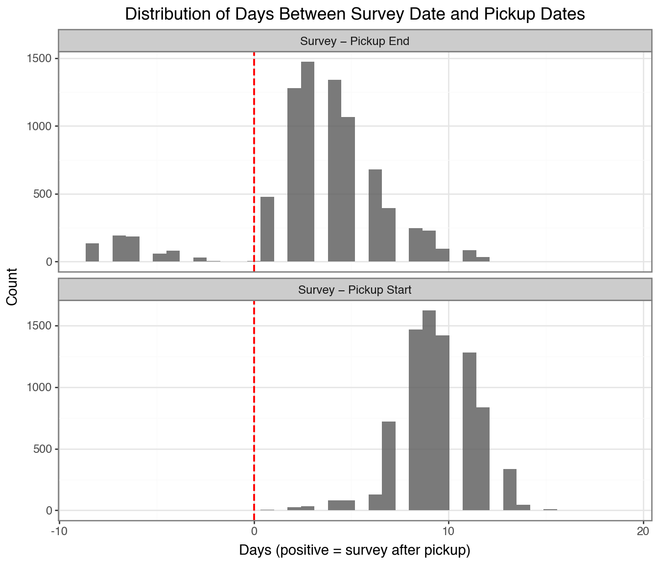
Below is a distribution of the difference in survey and pickup dates (in particular, the last pickup done).

Caution

The negative values indicate people who completed the survey BEFORE pickups were done. All of these happened due to the study pause in periods 3 (mostly) and period 4.

Code
```{python}
#| label: survey-pickup-dates
pickup = pd.read_stata(TIDY / "19_pickup-hh_id-period.dta")

# Merge survey_date from panel onto pickup (panel_df has survey_date; use full_panel_df before period filter)
survey_dates = full_panel_df[["hh_id", "period", "survey_date"]].copy()
survey_dates["period"] = survey_dates["period"].astype(int)
pickup["period"] = pickup["period"].astype(int)

pickup_merged = pickup.merge(survey_dates, on=["hh_id", "period"], how="left")
pickup_merged = pickup_merged[pickup_merged["period"] != 6].copy()

pickup_merged["days_to_pickup_end"]   = (pickup_merged["survey_date"] - pickup_merged["pickup_end"]).dt.days
pickup_merged["days_to_pickup_start"] = (pickup_merged["survey_date"] - pickup_merged["pickup_start"]).dt.days

pickup_merged.to_stata(PROJ_ROOT / "PICKUP_DIAG.dta", write_index=False)

# Summary table
summary = pickup_merged[["days_to_pickup_end", "days_to_pickup_start"]].describe().round(1)
summary.columns = ["Survey − Pickup End (days)", "Survey − Pickup Start (days)"]
```
Code
```{python}
#| label: survey-pickup-histograms
plot_days = pickup_merged[["days_to_pickup_end", "days_to_pickup_start"]].melt(
    var_name="measure", value_name="days"
).dropna()
plot_days["measure"] = plot_days["measure"].map({
    "days_to_pickup_end":   "Survey − Pickup End",
    "days_to_pickup_start": "Survey − Pickup Start",
})

(
    ggplot(plot_days, aes(x="days"))
    + geom_histogram(bins=40, alpha=0.8)
    + geom_vline(xintercept=0, linetype="dashed", color="red", size=0.8)
    + facet_wrap("measure", ncol=1, scales="free_y")
    + theme_bw()
    + labs(x="Days (positive = survey after pickup)", y="Count",
           title="Distribution of Days Between Survey Date and Pickup Dates")
    + theme(figure_size=(7, 6), strip_text=element_text(size=9))
)
```

Code
```{python}
#| label: predictable-timing-setup
# 1. Store median days_to_pickup_end
median_days_to_pickup_end = pickup_merged["days_to_pickup_end"].median()

# 2. Merge days_to_pickup_end onto panel_df (one row per hh_id-period)
pickup_days = (
    pickup_merged[["hh_id", "period", "days_to_pickup_end"]]
    .drop_duplicates(subset=["hh_id", "period"])
)
panel_df = panel_df.merge(pickup_days, on=["hh_id", "period"], how="left")

# 3. Create arm_predictable:
#    - "Control"            if treatment == 0
#    - "Predictable Early"  if treatment == 2 and days_to_pickup_end <= median
#    - "Predictable Late"   if treatment == 2 and days_to_pickup_end >  median
#    - NaN                  for all other treatments
def _arm_predictable(row):
    if row["treatment"] == 0:
        return "Control"
    elif row["treatment"] == 2:
        if pd.isna(row["days_to_pickup_end"]):
            return np.nan
        return (
            "Predictable Early"
            if row["days_to_pickup_end"] <= median_days_to_pickup_end
            else "Predictable Late"
        )
    return np.nan

def _arm_stable(row):
    if row["treatment"] == 0:
        return "Control"
    elif row["treatment"] == 3:
        if pd.isna(row["days_to_pickup_end"]):
            return np.nan
        return (
            "Stable Early"
            if row["days_to_pickup_end"] <= median_days_to_pickup_end
            else "Stable Late"
        )
    return np.nan

panel_df["arm_predictable"] = panel_df.apply(_arm_predictable, axis=1)
panel_df["arm_stable"] = panel_df.apply(_arm_stable, axis=1)

panel_df["arm_predictable"] = pd.Categorical(
    panel_df["arm_predictable"],
    categories=["Control", "Predictable Early", "Predictable Late"],
)

panel_df["arm_stable"] = pd.Categorical(
    panel_df["arm_stable"],
    categories=["Control", "Stable Early", "Stable Late"],
)

# Subset: phone survey periods only, drop rows with no arm assignment
predictable_timing_df = panel_df[
    (panel_df["period"] > 0) &
    (panel_df["period"] < 6) &
    panel_df["arm_predictable"].notna()
].copy()

stable_timing_df = panel_df[
    (panel_df["period"] > 0) &
    (panel_df["period"] < 6) &
    panel_df["arm_stable"].notna()
].copy()
```

Restricting to the predictable arm, let us see if it makes a difference

Note

Median date used to split predictable arm is 4 days. It is done at the period level so people could switch in and out of the below/above median split over time.

Code
```{python}
#| label: predictable-timing-cdf
PALETTE_PREDICTABLE = {
    "Control":           "#333333",
    "Predictable Early": "#2196F3",
    "Predictable Late":  "#E91E63",
}

(
    ggplot(
        predictable_timing_df.dropna(subset=["food_purchase_total_99_ae_resid"]),
        aes(x="food_purchase_total_99_ae_resid", color="arm_predictable"),
    )
    + stat_ecdf(size=0.9)
    + scale_color_manual(values=PALETTE_PREDICTABLE, name="Arm")
    + labs(
        x="Food Purchases Per Adult Equivalent (residualized)",
    )
    + theme_minimal()
    + theme(figure_size=(6, 4), legend_position="right")
)
```

Code
```{python}
#| label: stable-timing-cdf
PALETTE_STABLE = {
    "Control":           "#333333",
    "Stable Early": "#2196F3",
    "Stable Late":  "#E91E63",
}

(
    ggplot(
        stable_timing_df.dropna(subset=["food_purchase_total_99_ae_resid"]),
        aes(x="food_purchase_total_99_ae_resid", color="arm_stable"),
    )
    + stat_ecdf(size=0.9)
    + scale_color_manual(values=PALETTE_STABLE, name="Arm")
    + labs(
        x="Food Purchases Per Adult Equivalent (residualized)",
    )
    + theme_minimal()
    + theme(figure_size=(6, 4), legend_position="right")
)
```

Appendix

All CDFs

CDFs for all outcomes and arms are available here: CDFs