March 17, 2026 - Analysis Wk.2: CDFs

Published

March 10, 2026

Abstract

Lumpiness and IDI-based analysis

Summary of Last Week

Discussed on March 10, 2026. Meeting notes available here.

Big Takeaways: - No clear pattern from the CDFs - We decided to take a look at the lumpiness of food purchases and try to think about the gap between respondents reported income and expenditure

Analysis for this week: - Explore IDIs - Lumpiness of food purchases

Lumpiness

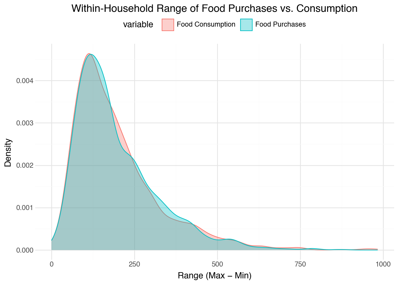
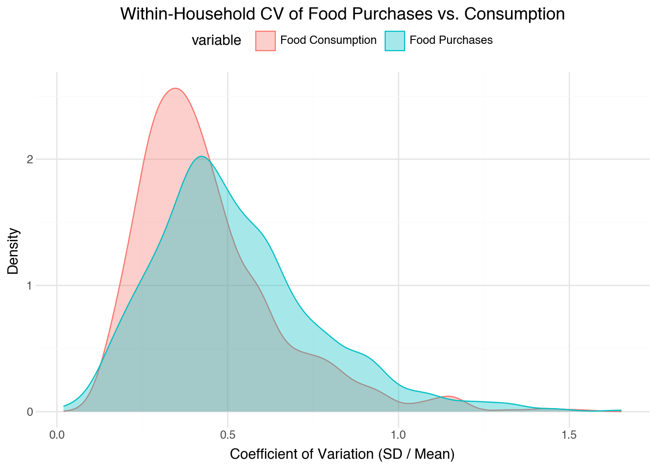
The graphs below plot the volatility of food purchases side by side with consumption. I include graphs of consumption to serve as a reference, since the assumption is that consumption should be smoother than food purchases given that household consume from their stock of food.

Large differences in the volatility of food purchases would be a potential indicator of lumpiness: households being a lot of food in one period and then not purchasing much in others while maintaining a smooth consumption.

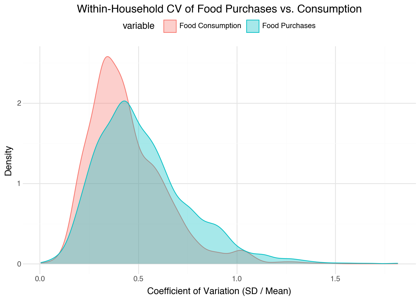
The figures below indicate that there might be some lumpiness, but not a lot. The range between the two is fairly close, making the large purchases of food not likely. However, the CV is larger which is consistent with the story that people consume more of their own produce and / or harvest to smooth consumption.

Risky and Predictable Arms
Control and Stable Arms

Code

```{python}
#| label: fig-range
#| fig-cap: Distribution of within-household range (max − min) for phone food purchases and phone food consumption.

range_df = (
    hh_df[hh_df["treatment"].isin([2, 3])][["purchase_range", "consumption_range"]]
    .melt(var_name="variable", value_name="range")
    .dropna()
    .assign(variable=lambda d: d["variable"].map({
        "purchase_range": "Food Purchases",
        "consumption_range": "Food Consumption"
    }))
)

(
    ggplot(range_df, aes(x="range", fill="variable", color="variable"))
    + geom_density(alpha=0.35)
    + labs(
        title="Within-Household Range of Food Purchases vs. Consumption",
        x="Range (Max − Min)",
        y="Density",
        fill=None,
        color=None,
    )
    + theme_minimal()
    + theme(legend_position="top")
)
```

Figure 1: Distribution of within-household range (max − min) for phone food purchases and phone food consumption.

Code

```{python}
#| label: fig-cv
#| fig-cap: Distribution of within-household coefficient of variation (SD / Mean) for phone food purchases and phone food consumption.

cv_df = (
    hh_df[hh_df["treatment"].isin([2, 3])][["purchase_cv", "consumption_cv"]]
    .melt(var_name="variable", value_name="cv")
    .dropna()
    .assign(variable=lambda d: d["variable"].map({
        "purchase_cv": "Food Purchases",
        "consumption_cv": "Food Consumption"
    }))
)

(
    ggplot(cv_df, aes(x="cv", fill="variable", color="variable"))
    + geom_density(alpha=0.35)
    + labs(
        title="Within-Household CV of Food Purchases vs. Consumption",
        x="Coefficient of Variation (SD / Mean)",
        y="Density",
        fill=None,
        color=None,
    )
    + theme_minimal()
    + theme(legend_position="top")
)
```

Figure 2: Distribution of within-household coefficient of variation (SD / Mean) for phone food purchases and phone food consumption.

Code

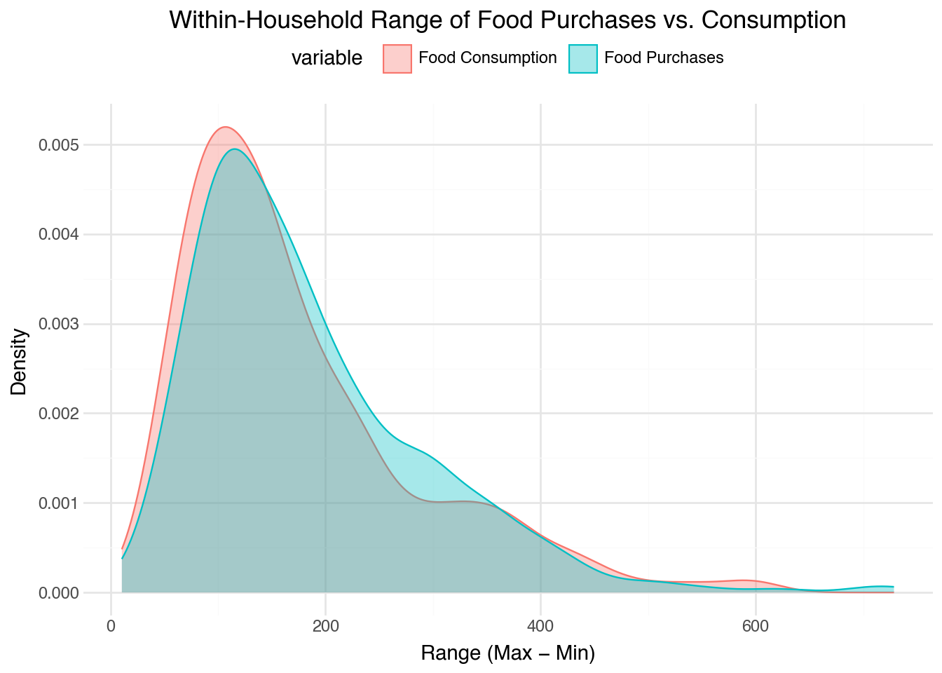
```{python}
#| label: fig-range-stable
#| fig-cap: Distribution of within-household range (max − min) for phone food purchases and phone food consumption.

range_df = (
    hh_df[hh_df["treatment"].isin([0, 1])][["purchase_range", "consumption_range"]]
    .melt(var_name="variable", value_name="range")
    .dropna()
    .assign(variable=lambda d: d["variable"].map({
        "purchase_range": "Food Purchases",
        "consumption_range": "Food Consumption"
    }))
)

(
    ggplot(range_df, aes(x="range", fill="variable", color="variable"))
    + geom_density(alpha=0.35)
    + labs(
        title="Within-Household Range of Food Purchases vs. Consumption",
        x="Range (Max − Min)",
        y="Density",
        fill=None,
        color=None,
    )
    + theme_minimal()
    + theme(legend_position="top")
)
```

Figure 3: Distribution of within-household range (max − min) for phone food purchases and phone food consumption.

Code

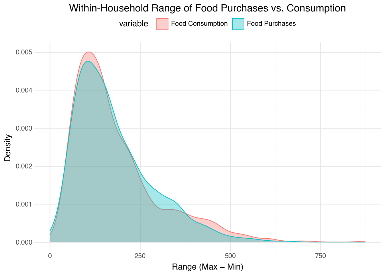
```{python}
#| label: fig-cv-stable
#| fig-cap: Distribution of within-household coefficient of variation (SD / Mean) for phone food purchases and phone food consumption.

cv_df = (
    hh_df[hh_df["treatment"].isin([0, 1])][["purchase_cv", "consumption_cv"]]
    .melt(var_name="variable", value_name="cv")
    .dropna()
    .assign(variable=lambda d: d["variable"].map({
        "purchase_cv": "Food Purchases",
        "consumption_cv": "Food Consumption"
    }))
)

(
    ggplot(cv_df, aes(x="cv", fill="variable", color="variable"))
    + geom_density(alpha=0.35)
    + labs(
        title="Within-Household CV of Food Purchases vs. Consumption",
        x="Coefficient of Variation (SD / Mean)",
        y="Density",
        fill=None,
        color=None,
    )
    + theme_minimal()
    + theme(legend_position="top")
)
```

Figure 4: Distribution of within-household coefficient of variation (SD / Mean) for phone food purchases and phone food consumption.

Category Breakdown

Another approach to investigating lumpiness is to look at the category breakdown of food purchases and comparing perishable categories, like meat and fruits, to grains and pulses. Unfortunately, the spend on those category is very low with the 75% percentile being 50 or less for meat, veges, and fruits.

Food Purchases and Food Insecurity

Code

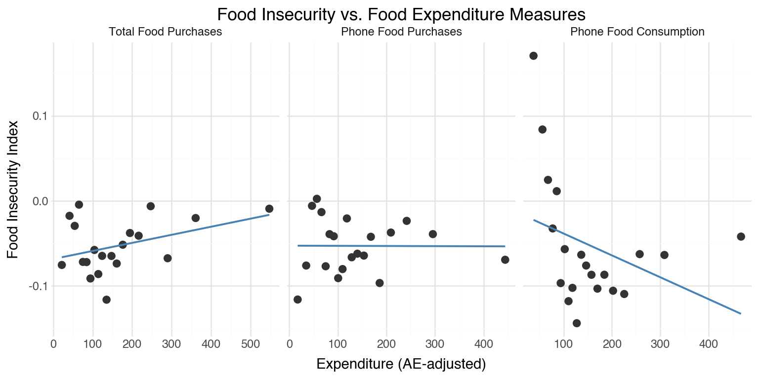
```{python}
#| label: food-insecurity
#| fig-cap: Binscatter of food insecurity index against food expenditure measures (20 equal-frequency bins, OLS fit line).

def binscatter(df, x_var, y_var, n_bins=20):
    """Stata-style binscatter: bin x into n equal-frequency bins, return mean(x) and mean(y) per bin."""
    tmp = df[[x_var, y_var]].dropna().copy()
    tmp["bin"] = pd.qcut(tmp[x_var], q=n_bins, labels=False, duplicates="drop")
    return (
        tmp.groupby("bin")
        .agg(x_mean=(x_var, "mean"), y_mean=(y_var, "mean"))
        .reset_index(drop=True)
    )

vars_to_plot = [
    ("food_purchase_total_99_ae",       "Total Food Purchases"),
    ("food_purchase_total_phone_99_ae",  "Phone Food Purchases"),
    ("food_consumption_phone_99_ae",     "Phone Food Consumption"),
]

bins_list = []
for var, label in vars_to_plot:
    bd = binscatter(panel_df, var, "fi_index")
    bd["x_label"] = label
    bins_list.append(bd)

bins_df = pd.concat(bins_list, ignore_index=True)
bins_df["x_label"] = pd.Categorical(
    bins_df["x_label"],
    categories=[l for _, l in vars_to_plot],
    ordered=True
)

(
    ggplot(bins_df, aes(x="x_mean", y="y_mean"))
    + geom_point(size=2.5, color="#333333")
    + geom_smooth(method="lm", se=False, color="steelblue", size=0.8)
    + facet_wrap("x_label", scales="free_x", nrow=1)
    + labs(
        title="Food Insecurity vs. Food Expenditure Measures",
        x="Expenditure (AE-adjusted)",
        y="Food Insecurity Index",
    )
    + theme_minimal()
    + theme(figure_size=(8, 4))
)
```

Binscatter of food insecurity index against food expenditure measures (20 equal-frequency bins, OLS fit line).

Code

```{python}
#| label: food-insecurity-regs
#| output: asis
import statsmodels.formula.api as smf
import warnings
from stargazer.stargazer import Stargazer
from IPython.display import HTML
warnings.filterwarnings("ignore")

reg_df = panel_df.dropna(subset=["fi_index"]).copy()
reg_df["period_str"] = reg_df["period"].astype(str)

# Divide all the expenditure variables by 1000 to make the coefficients more interpretable
for var in ["food_purchase_total_99_ae", "food_purchase_total_phone_99_ae", "food_consumption_phone_99_ae"]:
    reg_df[var] = reg_df[var] / 100

specs = [
    ("fi_index ~ food_purchase_total_99_ae",                 "food_purchase_total_99_ae"),
    ("fi_index ~ food_purchase_total_99_ae + C(period_str)", "food_purchase_total_99_ae"),
    ("fi_index ~ food_purchase_total_phone_99_ae + C(period_str)", "food_purchase_total_phone_99_ae"),
    ("fi_index ~ food_consumption_phone_99_ae + C(period_str)",    "food_consumption_phone_99_ae"),
]

fitted = [smf.ols(f, data=reg_df).fit(cov_type="HC3") for f, _ in specs]

sg = Stargazer(fitted)
sg.title("Food Insecurity vs. Food Expenditure Measures")
sg.custom_columns(
    ["(1) Food Purchases", "(2) + Period FEs",
     "(3) Phone Purchases + FEs", "(4) Phone Consumption + FEs"],
    [1, 1, 1, 1]
)
sg.covariate_order([
    "food_purchase_total_99_ae",
    "food_purchase_total_phone_99_ae",
    "food_consumption_phone_99_ae",
])
sg.rename_covariates({
    "food_purchase_total_99_ae":       "Food Purchases (AE)",
    "food_purchase_total_phone_99_ae": "Phone Food Purchases (AE)",
    "food_consumption_phone_99_ae":    "Phone Food Consumption (AE)",
})
sg.add_line("Period FEs", ["No", "Yes", "Yes", "Yes"])
sg.show_degrees_of_freedom(False)

sg
```

Food Insecurity vs. Food Expenditure Measures


	Dependent variable: fi_index

	(1) Food Purchases	(2) + Period FEs	(3) Phone Purchases + FEs	(4) Phone Consumption + FEs
	(1)	(2)	(3)	(4)

Food Purchases (AE)	0.009^**	0.001
	(0.005)	(0.005)
Phone Food Purchases (AE)			-0.006
			(0.006)
Phone Food Consumption (AE)				-0.031^***
				(0.006)
Period FEs	No	Yes	Yes	Yes

Observations	14827	14827	14827	14827
R²	0.000	0.002	0.003	0.004
Adjusted R²	0.000	0.002	0.002	0.004
Residual Std. Error	0.717	0.716	0.716	0.715
F Statistic	3.881^**	5.262^***	5.390^***	8.747^***

Note:	^p<0.1; ^p<0.05; ^**p<0.01

IDIs

I read through 3 IDIs to get a sense of what is going on.

Broad themes I noticed are

Income Sources

Debt

3 / 6 IDIs I skimmed mention borrowing to fund their agriculture
- eg. buy fertilizer, herbicide
Respondents mention paying off debt as a large source of stress
- Not sure if their harvests will be good enough to pay off their debt
- Even after harvest, they might not have a lot left for themselves
2 treated respondents mentioned having bag work allowed them to borrow more
- Both respondents and lenders felt more confident they would be able to pay back their loans (according to respondents)

Little Work

Only 1 IDIs mention labor that is paid
Mostly mention selling some produce or ground nuts
- They also mention smoothing consumption by selling groundnuts but then buying it later
Livestock to cover emergenices (funeral costs, sickness, etc.)

Little no smoothing

Control group mentions having almost no extra cash for emergencies or other discretionary spending
- Might be coincidence but 2/3 mention an ae that required treatment and stress around paying for expenses
In the predictable and risky I read, they both mention consuming earnings directly that period.
Because of this an the lack of work aforementioned, people seemed to really appreciate the bags. Some frustration around low draws but my read of the interview gave me the sense that having some disposable was very valuable but it felt having more had dimishsing returns (note: this is my interpretation and the respondents did say they would have preferred to ahve more)
Our endline measures of financial insecurity don’t capture this distinction. Potentially due to the working being over

Less in control (if that is the case) might just relfect that they couldn’t borrow

Harvest

Groundnut harvest doesn’t seem to have been great. It seemed that the rains started then stopped which might have caused some issue
- It seemed early planters were hurt
Maize harvests were only beginning
Mentions of drought and not great rains. In all the IDIs it seems respondents were concerned about their yields
- They did universally say it was better than last year

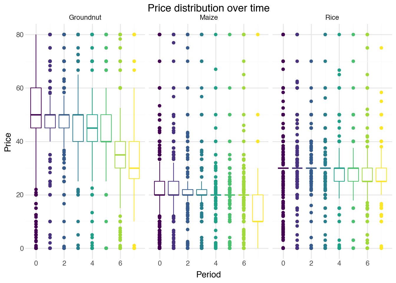
Prices

One respondent mentioned that rice got more expensive while the others said that maize got cheaper
Others say no change

Data shows things are somewhat stable with a bit of deflation

Code

```{python}
food_data_purchases = food_data[food_data["type"] == "purch"].copy()
food_purchase_prices = food_data_purchases[food_data_purchases["item_unique_id"].isin([24, 30, 48])][["period", "item_unique_id", "total_cost", "unit", "total_qty"]]
food_purchase_prices = food_purchase_prices[food_purchase_prices["unit"] == 8]
food_purchase_prices["price"] = food_purchase_prices["total_cost"] / food_purchase_prices["total_qty"]
p99_price = food_purchase_prices["price"].quantile(0.99)
food_purchase_prices["price"] = food_purchase_prices["price"].clip(lower=0, upper=p99_price) 
food_purchase_prices["item"] = food_purchase_prices["item_unique_id"].map({
    24: "Groundnut",
    30: "Maize",
    48: "Rice"
})

food_purchase_prices = food_purchase_prices[food_purchase_prices["price"].notna()]

(
    ggplot(food_purchase_prices, aes(x="period", group="period", y="price", color="period"))
    + geom_boxplot()
    + facet_wrap("item", nrow=1)
    + labs(
        title="Price distribution over time",
        x="Period",
        y="Price",
        fill=None,
        color=None,
    )
    + theme_minimal()
    + theme(legend_position="none")
)
```